


III. BAIHP Research C
BAIHP builds on a 20 year foundation of basic building science research at the Florida Solar Energy Center. This research generally focuses on issues important in hot-humid climates similar to Florida’s but is relevant to our understanding of building science concepts manifest in all climatic regions. BAIHP has conducted field and laboratory building science research in these areas:
Air
Handler Air Tightness Study
Central Florida
Research by FSEC Researchers Chuck Withers, Jim Cummings, and Janet McIlvaine
Papers: Cummings, J.,
C. Withers, J. McIlvaine, J. Sonne, M. Lombardi (2003). Air Handler Leakage:
Field Testing Results in Residences. ASHRAE Transactions V.109 pt.1 February
2003. To be published in ASHRAE Journal.
To determine the impact of air handler location on heating and cooling energy use, researchers measured the amount of air leakage in air handler cabinets, and between the air handler cabinet and the return and supply plenums. To assess this leakage, testing was performed on 69 air conditioning systems. Thirty systems were tested in the 2001 and 39 in 2002. The 69 systems were tested in 63 Florida houses (in six cases, two air handlers were tested in a single house) located in seven counties across the state - four in Leon County in or near Tallahassee, 17 in Polk County, three in Lake County, 13 in Orange County, one in Osceola County, two in Sumter County, and 29 in Brevard County. All except those in Leon County are located in central Florida. Construction on all houses was completed after January 1, 2001, and most homes were tested within four months of occupancy.
In each case, air leakage (Q25) at the air handler and two adjacent connections was measured. Q25 is the amount of air leakage which occurs when the ductwork or air handler is placed under 25 Pa of pressure with respect to its surrounding environment. Q25 also can be considered a measurement of ductwork perforation.
To obtain actual air leakage while the system operated, it was necessary to measure the operating pressure differential between the inside and outside of the air handler and adjacent connections. In other words, it was necessary to know the perforation or hole size and the pressure differential operating across that hole. By determining both Q25 and operating pressure differentials, actual air leakage into or out of the system was calculated.
Field Testing Leakage Parameters
Testing was performed on 69 air conditioning systems to determine the extent
of air leakage from air handlers and adjacent connections. Testing and
inspection was performed to obtain:
- Q25 in the air handler, Q25 at the connection to the return plenum, and Q25 at the connection to the supply plenum.
- Operating pressure at four locations - the return plenum connection, in the air handler before the coil, in the air handler after the coil, and at the supply plenum connection.
- Return and supply air flows were measured with a flow hood. Air handler flow rates were measured with an air handler flow plate device (per ASHRAE Standard 152P methodology).
- Overall duct system and house air tightness in 20 of the 69 homes.
- Cooling and heating system capacity based on air handler and outdoor unit model numbers.
- The location and type of filter.
- Dimensions and surface area of the air handler cabinet.
- The fractions of the air handler under negative pressure and under positive pressure.
- The types of sealants used at air handler connections.
- Estimated portion of the air handler leak area that was sealed “as found."
Air Handler Leakage
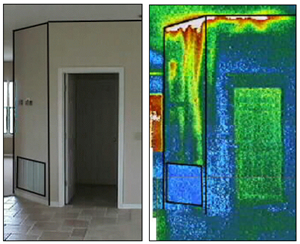 |
Figure 92. Thermograph of air being
drawn from the attic to the air handler in a Florida house |
Leakage in the air handler cabinet averaged 20.4 Q25 in 69 air conditioning systems. Leakage at the return and supply plenum connections averaged 3.9 and 1.6 Q25, respectively. Using the operating pressures in the air handler and at the plenum connections, these Q25 results convert to actual air leakage of 58.8 CFM on the return side (negative pressure side) and 9.3 CFM on the supply side (positive pressure side). The combined return and supply air leakage in the air handler and adjacent connections represents 5.3% of the system air flow (4.6% on the return side and 0.7% on the supply side). This is a concern, when considering that a 4.6% return leak from a hot attic (peak conditions; 120oF and 30% RH) can produce a 16% reduction in cooling output and 20% increase in cooling energy use (Cummings and Tooley, 1989), and this was only from the air handler and adjacent connections. (Figure 92)
“Total” Duct Leakage
Some important observations were made from the extended test data in 20 houses.
Total leakage on the return side of the system (including the air handler and
return connection) was 53 cfm with weighted operating pressure on the return
side of about -100 Pa (including the air handler), operating return leakage
was calculated to be 122 CFM, or 9.7% of the rated system air flow.
Total leakage on the supply side of the system (Q25s,total) was very large,
at 134. The ASHRAE 152P method suggests using half of the supply plenum pressure
as an estimate of the overall supply ductwork operating pressure, if the
actual duct pressures are not known. For the 20 systems with extended testing,
supply plenum pressure was 73.3 Pa. Based on a pressure of 37 Pa, actual
leakage should be 167 CFM or about 13.3% of the rated air flow. To test the
ASHRAE divide-by-two method, supply duct operating pressure measurements
were taken from 14 representative systems. These averaged 35.9 Pa, compared
to 65.7 Pa for the supply plenums for those same 14 systems. For these systems,
the duct pressure was 55% of the supply plenum pressure - making the ASHRAE
method a reasonable method for estimating central Florida home’s supply ductwork operating pressures.
However, the ASHRAEmethod wasn’t reasonable for estimating central Florida home’s return ductwork operating pressures. For these 20 systems, 38% of the Q25r,total was in the air handler and 62% of the Q25r,total was in the return ductwork. Given an air handler pressure of -133 Pa, a return plenum pressure of -81.5 Pa, and return duct pressure of approximately -70 Pa, the weighted return side pressure was approximately -95 Pa. By contrast, the ASHRAE method predicted -41 Pa. Clearly, in systems with a single, short return duct plenum like those commonly found in Florida, the actual operating pressure should be greater than the return plenum, maybe by as much as 1.2 times the plenum pressure.
Return side leakage is available on 58 of the 69 systems. Return leak air flow (Qr,total) combined for the air handler, return connection, and the return ductwork was found to be 152.4 CFM, or 11.8% of total rated system air flow for this group. For this larger sample, Qr,total is considerably greater than for the 20 houses with extended testing. These alarming results show that even in these newly constructed homes about 12% of return air and 13% of supply air duct systems are leaking.
Duct Leakage to “Out”:
In 20 homes, duct leakage to “out” was measured. (Table 63) On average, 56% of the leakage of the return ductwork and supply ductwork was to “out.” “Out” is defined as outside the conditioned space, including buffer spaces like an attic or garage. The fraction of leakage that was to “out” varied by air handler location. For return ductwork, the proportion of total leakage to “out” is 81.4% for attic systems, 67.6% for garage, and 28.0% for indoors. For supply ductwork, the proportion of total leakage to “out” was in the range of 52% to 56% for all three locations.
Table 63. Portion of duct leakage to outdoors [(Q25,out/Q25,total) * 100]
| Air Handler Location | Return | Supply | Entire Duct System |
| Attic | 81.4% | 56.5% | 63.2% |
| Garage | 67.6% | 51.7% | 56.0% |
| Indoors | 28.0% | 52.6% | 37.1% |
The attic return ductwork was the most predictive variable to “out” leakage findings. All of the return ductwork for attic units was located in the attic. Much of the return ductwork for other units was located in the house. As a consequence, the energy penalty associated with locating the air handler in the attic was greater than indicated in the computer modeling results in Table 64, since the modeling only considered the leakage of the air handler cabinet and the adjacent connections, and not the return ductwork leakage.
Table 64. Duct leakage “total” and to “out” for
three locations, for both 25 Pa test
pressure and for actual system operating
pressure. Sample size is in [brackets]
| Attic (cfm) | Garage (cfm) | Indoors (cfm) | Combined (cfm) | |||||
| Test | Total | Out | Total | Out | Total | Out | Total | Out |
| Q25,r [58] | 61.9 | 50.4 | 93.3 | 63.1 | 67.8 | 19.0 | 75.7 | 44.9 |
| Q25,s [20] | 109.1 | 61.6 | 170.6 | 88.2 | 119.5 | 62.9 | 134.3 | 71.4 |
| Qr [58] | 118.1 | 96.1 | 194.4 | 131.4 | 134.6 | 37.7 | 152.4 | 90.4 |
| Qs [20] | 135.6 | 76.6 | 212.0 | 109.6 | 148.5 | 78.1 | 166.9 | 88.7 |
Table 64 shows that the operating supply leakage to “out” was large for all three air handler locations, averaging 89 CFM. The average operating return leakage to “out” was slightly larger, at 90 CFM. However, there was a large variation between air handler locations; 96 CFM for attic systems, 131 CFM for garage systems, but only 38 CFM for indoor systems. From an energy perspective, the attic systems experienced the greatest “real” energy penalties, because all of the return ductwork and air handlers were located in the attic. (Table 63) By contrast, a majority of the return leakage for the garage systems likely came from the garage (which is considerably cooler than the attic). For indoor systems, the return leakage to “out” most likely originated from the attic. However, since the return leakage was so much smaller, the energy impact was likely considerably less than both the attic and the garage systems.
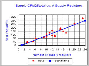
Correlation of Supply Duct Leaks with Number of Registers: When analyzing the supply leakage in the extended test data, a surprising correlation was observed. This correlation indicated a systematic and consistent duct fabrication problem across a wide range of air conditioning contractors. Figure 93 illustrates this correlation, showing that each supply duct has a remarkably predictable total duct leakage. The coefficient of determination is 0.86, indicating that 86% of the variability in total supply duct leakage was explainable by the number of supply registers. Figure 94 shows a similar relationship between supply leakage to “out” and the number of supply registers. In this case the coefficient of determination was 0.69, indicating that 69% of the variability in total supply duct leakage was explainable by the number of supply registers.
 |
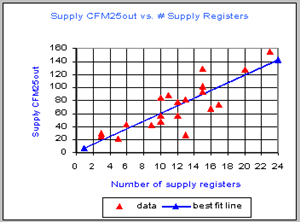 |
Figure 93. Supply
CFM25 “total” leakage versus the number of supply registers. |
Figure 94. Supply CFM25 “out” leakage versus the number of supply registers. |
Note that one of the two houses with 13 registers showed considerably less leakage than expected. In this case, supply ducts were located in the interstitial space between floors. When the house was taken to -25 Pa, it is probable (though not measured) that the interstitial spaces were substantially depressurized as well, so leaks in those supply ducts would show less air flow (i.e., less pressure differential = less leakage air flow) and therefore be under-represented.
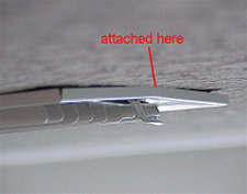 |
Figure 95. Gaps at the supply
register to drywall joint |
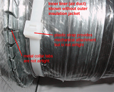 |
Figure 96. Flexible
duct to metal collar connection. |
The data suggest that a duct leakage problem occurs in nearly all new homes. Researchers identified three issues that create most of the leakage: (1) the connection of the supply register or return grill (Figure 95), (2) the boot (supply box) to sheet rock connection (Figure 96), and (3) the flex duct to collar connection. The supply register or return grill leakage typically shows as supply leakage in the “total” test. It usually occurs when the register or grill does not fit snugly to the ceiling or wallboard. Issues two and three show up as leakage to both “out” and “total.”
Figure 96 shows how flexible duct connections typically are made. In some cases metal tape is used, but the tape wrinkles when applied to complex angles and over bumps associated with these connection types. Although small in size, these cumulative wrinkles at each connection allow air to pass through.
Computer Modeling for Florida Energy Code Air Handler Multipliers:
FSEC researchers performed simulations and developed air handler multipliers for the Florida Energy Code using this study’s simulation results. Researcher used the FSEC 3.0 model, a general building simulation program developed in 1992. This program provided simultaneous detailed simulations of a whole building system, including energy, moisture, multi-zone air flows, and air distribution systems.
In 2001, modeling had been performed to develop initial air handler multipliers. These multipliers were based on estimated Q25 and duct operating pressures. At the time of the 2001 modeling, there was essentially no data on air handler and connection leakage. Modeling for this project was performed again, but this time using the results of the 69 field tested homes.
The modeling inputs used in 2001 and those from the current study are shown below. (Table 65) Note that the same Q25 and operating depressurization (dP) values was used for all air handler locations, since there was essentially no difference between the Q25 values for attic, garage, and indoor air handler locations when gas furnace units were removed from the analysis.
Table 65. Air Handler (AH) And Connection
Inputs For 2001
and
Current Project Computer Modeling
2001 Q25 |
AH Study Q25 |
2001 dP |
AH Study dP |
|
| Return connection | 8.7 |
3.9 |
-40 |
-86.1 |
| AH – depressurized portion | 48.5 |
17.6 |
-42 |
-139.1 |
| AH – pressurized portion | 9.6 |
2.8 |
43 |
106.5 |
| Supply connection | 7.8 |
1.6 |
32 |
58.2 |
| Total | 74.6 |
25.9 |
|
|
While the Q25 leakage for the air handler and connections was about 65% less than earlier estimates, operating pressures were much higher. The air handler multipliers based on the current computer modeling results are presented in Tables 66, 67, and 68. Modeling of air handler energy use also was performed for the air handlers located outdoors, despite the fact that no field data was collected for outdoor units. The modeling input parameters were the same as the other air handler locations as shown in Table 65. Note also that the air handler multipliers for the attic, indoors, and outdoors are normalized to the garage, since this location was considered the baseline. The final report for this study can be viewed online at: http://www.fsec.ucf.edu/bldg/pubs/cr1357/index.htm.
Table 66. Florida Energy Code AH Multipliers for South Florida
| AH Location | Winter | Summer | ||||
Old |
2001 |
new |
old |
2001 |
new |
|
| Attic | 1.04 |
1.15 |
1.12 |
1.04 |
1.09 |
1.06 |
| Garage | 1.00 |
1.00 |
1.00 |
1.00 |
1.00 |
1.00 |
| Indoors | 0.93 |
0.91 |
0.94 |
0.93 |
0.91 |
0.92 |
| Outdoors | 1.03 |
1.08 |
1.06 |
1.03 |
1.03 |
1.01 |
Table 67. Florida Energy Code AH Multipliers for Central Florida
| AH Location | Winter | Summer | ||||
Old |
2001 |
new |
old |
2001 |
new |
|
| Attic | 1.04 |
1.11 |
1.08 |
1.04 |
1.10 |
1.08 |
| Garage | 1.00 |
1.00 |
1.00 |
1.00 |
1.00 |
1.00 |
| indoors | 0.93 |
0.92 |
0.94 |
0.93 |
0.90 |
0.92 |
| outdoors | 1.03 |
1.09 |
1.05 |
1.03 |
1.02 |
1.01 |
Table 68. Florida Energy Code AH Multipliers for North Florida
| AH Location | Winter | Summer | ||||
Old |
2001 |
new |
old |
2001 |
new |
|
| attic | 1.04 |
1.10 |
1.03 |
1.04 |
1.11 |
1.08 |
| garage | 1.00 |
1.00 |
1.00 |
1.00 |
1.00 |
1.00 |
| indoors | 0.93 |
0.93 |
0.94 |
0.93 |
0.91 |
0.92 |
| outdoors | 1.03 |
1.07 |
1.02 |
1.03 |
1.02 |
1.01 |
Florida Solar Energy Center, Laboratory Facilities
Cocoa, Florida
Paper Parker, D., Sherwin, J., Hibbs, B., " Development of High Efficiency Air Conditioner Condenser Fans", Draft paper to be published in ASHRAE Transactions in June 2005.
Purpose
 |
Figure 97. Air conditioning condenser fan and diffuser |
The purpose of this study is to develop an air conditioner condenser fan that reduces the electric energy use of the condensing unit (Figure 97). To accomplish this, researchers are designing and producing more aerodynamic fan blades and substituting smaller horsepower (HP) motors which achieve the same air flow rates as the larger, less efficient motors typically used.
4th Budget Period
During the 4th budget period, researchers developed baseline data for the fan power use in a standard condensing unit (Trane 2TTR2036) and tested a new prototype design: “Design A5” with five asymmetrical blades
Baseline data included condenser airflow, motor power, sound levels, and condenser cabinet pressures. Test results favorably compared with the manufacturer’s test data. An experimental set of fan blades, “Design-A5,” designed for a 1/8 hp motor at 850 rpm was numerically created and then successfully produced using rapid prototyping. These prototype blades were substituted on the original condenser, and all test measurements were redone. Design-A5 was found to reduce power use by 20% (40 watts) with approximately equivalent airflow to the original condensing blade design.
5th Budget Period
During the 5th budget period, activities included re-calibration and improvement of the test equipment configuration, refinement of various designs, and patent filing.
Re-calibration and Improvement of Test Equipment Configuration
The air flow measurement equipment was re-calibrated by the Energy Conservatory in Minneapolis in accordance with ANSI/ASHRAE 51-1985 ("Laboratory Methods of Testing Fans for Rating."). Testing determined that the "flow cube" could be modified with settling screens and a flow straightener to yield a 5% absolute flow accuracy and a 2% relative accuracy from the test equipment. Also, the test configuration was moved indoors in order to better measure sound and also to reduce test variability from wind-related effects. Noise measurement protocol improved to comply with procedures used by the air conditioning industry.
Continued Testing to Refine the Identified Condenser Fan and Condenser Top Design
All fans were re-evaluated after bringing the test apparatus into compliance with ANSI/ASHRAE 51-1985 ("Laboratory Methods of Testing Fans for Rating.") New fan prototypes “Design-D” and “Design E” were tested as well as a diffuser for a 27" fan and a specially prepared Electronically Commutated Motor (ECM) provided by General Electric.
All designs were also tested with the conical diffuser with 20-27% increases in measured flow from the low rpm designs, which use 8-pole motors. Sound measurements (Table 66) also showed large advantages with as much as a 4 dB reduction in fan sound level over the standard fan. The final test prototype with diffuser and fan is shown in Figure 98.
Table 66. Sound Measurements For Various Fan And Housing Designs
| Top | Fan | Motor | Flow | Power | Sound |
| OEM/ Starburst | OEM | 6-pole | 2170 cfm | 197 W | 63.0 dB |
| OEM-Foam | OEM | 6-pole | 2230 cfm | 198 W | 63.0 db |
| Wire top | OEM | 6-pole | 2180 cfm | 188 W | 62.0 dB |
| Wire-Foam | OEM | 6-pole | 2250 cfm | 190 W | 62.0 db |
| OEM-foam | A5 | 8-pole | 1945 cfm | 145 W | 62.0 dB |
| Wire-foam | A5 | 8-pole | 2110 cfm | 146 W | 60.0 dB |
| WhisperGuard w/foam | A5 | 8-pole | 2300 cfm | 143 W | 58.5 dB |
Presentation and Commercialization
In January, BAIHP researcher Danny Parker made a presentation at the DOE Expert meeting on HVAC and Fans in Anaheim, California and participated in productive meetings with Trane Corporation in May 2004 to discuss licensing of the technology under an existing non-disclosure agreement.
Patents Pending
U.S. Application Serial No. 10/400,888, Provisional applications 60/369,050 / 60/438,035 & UCF-449CIP; WhisperGuard (UCF-Docket No. UCF-458)
Key Improvements from WhisperGuard Technology
Tested Performance with Trane TTR2036 Condenser:
-
Provides 46 Watt reduction in fan power (144 W vs. 190 Watts)
-
Increases condenser air flow by 130 cfm (6% increase in fan flow)
-
Provides 102 W power reduction with ECM 142 motor
-
Reduce ambient fan-only sound level by 4-5 dB
-
ECM motor allows lower fan speeds for ultra-quiet night operation, higher flows for maximum capacity during very hot periods (temperature based control)
-
Attractive hi-tech diffuser appearance
Key Technologies Employed
-
High efficiency 5-bladed asymmetrical fan moves air quietly at lower fan speeds
-
Diffuser top for effective pressure recovery increasing air flow at slow speed ranges
-
Conical center body reduces exhaust swirl
-
Acoustic sound control strip to reduce tip losses and control tip vortex shedding
Final Year of the Project
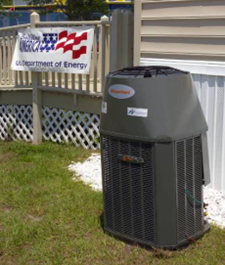 |
Figure 98. Final test prototype
with diffuser and fan. |
A detailed research paper on the progress on the condenser fan research and associated findings has been published within the ASHRAE Summer 2005 transactions and also is now published on-line. The paper was presented to a large audience in Denver at the meeting. The meeting was well attended by many HVAC manufactures. Both Lau Corp and Morrison Industries (large fan manufacturers for the AC industry) showed interest.
Work has been completed on larger 27.6" fans which will provide better performance for higher performance equipment (SEER 14+) with larger condensers. Detailed testing was performed on a 4-bladed fan with an annular diffuser with both PSC and ECM motors. Good results were obtained: 4580 cfm at 202 Watts against 4260 cfm and 244 Watts in the baseline configuration. Multiple tests with the ECM motors were obtained in April. We also produced a shorter diffuser for test which showed little compromise to air moving performance. With the ECM motor we obtained results with equivalent flow to the original test condition (4260 cfm at 244 watts) with only 147 Watts– almost a hundred watt power reduction (40% reduction in motor power). A version of this fan and assembly was delivered to California for their work on a hot-arid climate air conditioner. It is being tested in laboratories at Southern California Edison, however testing of the unit is not expected before November 2005 due to scheduling issues.
After describing performance to industry last summer, we are entering into discussions with Freus Air Conditioning about creating a fan with this advanced evaporatively pre-cooled air conditioner. Current fan power is on the order of 120 Watts. We expect we can reduce this by 30-50% with improved fan and exhaust section design. We have begun discussion with Rocky Bacchus regarding potential experimentation.
Florida Solar Energy Center, Laboratory Facilities
Cocoa, Florida
Research by BAIHP Researcher Ross McCluney
Fenestration: Windows & Daylighting Website
In the 6th budget period major revisions and additions were made to this website, located at http://www.fsec.ucf.edu/bldg/active/fen/index.htm.
Website
The website is now an effective education tool, and will help the consumer make informed, quality decisions concerning the technologies available for existing and new windows.
Work continues on the web site’s Decision Tree, which, when complete, will be an interactive process to guide the consumer through a number of questions, providing the specifics for a particular application. At the end, a report will be prepared giving recommendations for the specifications to be used in selecting the correct combination of windows and/or shades for the windows in the home. An Oracle Forms runtime file has been completed and illustrations readied.
AWNSHADE 3.0 Software Revision
AWNSHADE was given an extensive revision, making it a fully Windows-compatible computer program. It is available online as a beta version. The program facilitates the calculation of solar heat gain through vertical windows having exterior shading surfaces, using overhangs, awnings, sidewalls, or a combination.
ASAP Ray Tracing
The focus of this work is toward quantifying edge and other effects associated with Dr. McCluney’s previously published model for solar heat gain through planar interior shades attached to single and double pane glazing systems. Other assumptions used to create the model will also be analyzed. In this way, the magnitude of the errors in those assumptions can be quantified, and perhaps the model improved.
A Visual Basic program to calculate the transmittance of a parallel plate of glass as a function of incidence angle was completed and used to generate glass transmittance data for comparison with results of ASAP ray trace calculations of this same quantity. The ray traces were completed and the Fresnel calculations and ray trace results were compared. The two different methods of calculation yielded plots that are indistinguishable, providing confirmation that the ray tracing methodology is completely equivalent to the results of exact calculations using the Fresnel Equations.
ASAP ray trace simulations of both specular and diffuse reflection from a planar shade behind a single pane glazing at any angle of incidence were made. Considerable effort was expended to get the traces of both the specular and diffuse shade cases running properly and plotting results as a function of the ratio of shade width to spacing from the glazing.
Measured data from David Tait will be compared with the model predictions and with the ray trace results. This data is the result of some calorimeter measurements of the solar heat gain coefficient for various glazings plus interior planar shade combinations, as well as the properties of the glazings and shades needed to perform the calculations of McCluney/Mills interior shade solar heat gain algorithm.
We continued ray tracing work on the solar transmittance through a glazing and interior shade and succeeded in setting up a loop over the aspect ratio (shade width divided by the glass-to-shade gap spacing) for a given reflectance. This was repeated for different reflectances. The results of these and additional ray traces will be used to assess the assumptions used in the original model and to improve the model where needed.
The diffuse and specular shade files were run for a range of reflectances from 0.9 down to 0.2. The results show that the specular model is not as terrible as its over-simplifications might indicate, as long as the aspect ratio is above a certain set of values.
Future work includes searching for ways to improve the model, especially at high shade reflectance values. We will look at the edge effects more closely and improve the analytical model at smaller aspect ratios. The results will be presented in a technical paper to be submitted to ASHRAE for publication later this year or early 2006. The timing of this additional work was extended, due to Dr. McCluney’s semi-retirement from the university.
American Society of Heating, Refrigerating, and Air Conditioning Engineers (ASHRAE) Technical Committee
In 2002, BAIHP researchers wrote a statement of work for the development of a methodology to calculate solar spectral distributions incident on windows for various sun positions and atmospheric conditions. ASHRAE approved the project and sent it out for bid. Completion of this work project should make it much easier to determine the true solar heat gain through spectrally selective fenestration systems for varying atmospheric conditions and solar altitude angles.
Calorimetric Measurements of Complex Fenestration Systems
FSEC’s research calorimeter will be used both indoors with the FSEC Vortek solar simulator and outside under natural solar radiation, on its Sagebrush solar tracker, for window solar heat gain experiments. The results of this testing will offer a way to test the solar gain properties of complex and other non-standard fenestration options for industrialized housing, such as exterior and interior shades and shutters, and those placed between the panes of double pane windows.
Sagebrush Solar Tracker
The computer program running the calorimeter, the Sagebrush tracker, and both together is complete. It contains a user-friendly graphic interface and offers a wide variety of experimental opportunities. There are many channels for adding additional temperature sensors and the calorimeter/tracker can be operated with either the sun as a source - in a variety of tracking modes - or with FSEC’s Vortek solar simulator.
To conduct outdoor testing, the Neslab chiller must be connected to the flow meter, the temperature sensors to the calorimeter, and the calorimeter mounted on the tracker. The Sagebrush tracker now is functional, responding properly to commands sent from the computer, rotating in altitude, and azimuth and stopping when the limit switches are encountered. A telescopic sight and level for positioning it outdoors in the proper orientation for accurate solar tracking has been designed and is near fabrication completion.
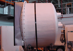 |
Figure 99. Side view of calorimeter
before it was mounted on the Sagebrush Tracker. |
The Neslab chiller and remote controller have been connected to a Gateway laptop computer and a RS-485 serial interface card necessary to operate the calorimeter has been installed. Researchers can now send commands and receive data from the chiller. Although the calorimeter is designed to work directly with the existing FSEC hydronic loop used for testing solar collectors, the Neslab will give an independent, standalone capability to the calorimeter. (Figure 99)
The water flow meter purchased for measuring the flow into the calorimeter has been successfully connected to the Agilent (HP) 34970A data acquisition system and its measurements were incorporated into the calorimeter operating program. Temperature sensors also successfully connected to the data acquisition system, are reading properly, and have been incorporated into the calorimeter program. The program has coding to include a number of additional temperature channels once the temperature probes have been received and installed in the calorimeter. Another 20-channel input card is being purchased for the Agilent, to permit additional temperature readings. Knowing the flow rate and temperature difference, the heat delivered to the water by the calorimeter can now be accurately determined.
Now that all portions of the system are operational, researchers will configure the outdoor system, verify, and begin testing in Year 5.
Vortek Solar Simulator
In 2003, the Vortek Simulator was fired up and operated reliably on the calorimeter testing with FSEC’s solar collector test apparatus. As expected, a few computer and other problems delayed initial data collection by a couple of days. However, these problems were corrected and testing proceeded normally.
During testing, the calorimeter was connected to the existing facility’s
hydronic loop, which was developed over a period of years to a temperature
stability of 0.01 degrees centigrade. The irradiance level measured about 820
watts per square meter over an aperture of 0.557 square meters. The calorimeter
was tested as though it were a flat plate collector, to obtain its efficiency
curve. This was used to infer the thermal losses and solar heat gain coefficient
of the eighth inch clear single pane of glass used for the test. The nominal
wind speed was set by the laminar blower to five miles per hour. The coolant
flow was run at levels of 0.2, 0.5, and 1.0 gallons per minute (GPM), and at
varying inlet temperatures.
For all test runs, steady state conditions were established by observing the
outlet temperature in a real-time plot as equilibrium was approached. During
periods of non-equilibrium, the recorded data was used to measure the first-order
system time constant, a function of the flow rate. The calorimeter time constant
varied from 1.5 minutes at 1.0 GPM to 6.9 minutes at 0.2 GPM. These time constants
were obtained by blocking the incident beam and watching the decay in outlet
temperature.
Skylight Dome Transmittance
Researchers completed work on the skylight dome transmittance, adding a spherical shape to the cylindrical one previously used. The ray tracing programming was changed to eliminate reflection of rays approaching the dome from the inside, for comparison with the analytical model, which does not yet include internal reflections. The difference between the two computational approaches, at a 30E solar zenith angle is 1.7%, considered acceptable for rating skylight performance.
With both cylindrical and spherical dome models, transmittance at large solar zenith angles above 60 is substantially greater than for a horizontal flat plate. This is because most of the rays incident on the dome and entering the skylight are incident on the dome close to perpendicular, where dome transmittance is highest.
EnergyGauge USA and EnergyGauge FlaRes
BAIHP mapped a table of window and shade characteristic simulations that could be run with these two programs. These runs will be used to determine the energy use of various fenestration options for Florida residences and to guide the preparation of instructional materials.
Florida Market Transformation
From the beginning of the BAIHP program, researchers have provided technical background information and support to the Alliance to Save Energy and the Efficient Windows Collaborative to promote the sale and installation of energy efficient fenestration in hot climates (such as Florida) and other areas for both conventional and industrialized homes. BAIHP also provides advice, technical information, and educational information to energy companies regarding window energy performance.
National Fenestration Rating Council (NFRC) Technical Committee
In 2002, BAIHP presented a final report at a Task Group meeting in Houston, on the NFRC- funded work to develop a draft standard practice for the rating of tubular daylighting devices. That project is now complete.
In 2001, BAIHP researchers performed a number of ray traces on a highly reflective cylinder of varying lengths, using the trace results to determine the cylinder’s transmittances for different interior surface reflectivities (from 90% to 100%). These results generated a “default table” for determining the transmittance of this tubular daylighting component. Using simplified assumptions, and then multiplying the tube transmittance by the top and bottom dome transmittance results, researchers determined the total transmittance for a chosen sun angle. Based on the findings, BAIHP provided NFRC and the industry with a list of suggested research projects to test and develop this methodology further. One of these submitted projects was sent out for bid by ASHRAE in Year 4 and is expected to begin in Year 5.
Tubular Daylighting Device SHGC and VT Value Calculations
Following a request from the TDD industry, a sequence of operations and a new computer program were written to access the Window 5 glazing database and obtain from it the spectral transmittance and front and back reflectance data for any sheet of glazing in that database which might be used in making the top dome of a tubular daylighting device. This permits determination of the input parameters needed to run TDDTrans. The computer program was posted for free download and is available by clicking on http://www.fsec.ucf.edu/bldg/active/fenestration/Software/Software_Download.htm
Access sequence:
-
Download and run the Optics 5 program.
-
Select the glazing to be used in the tubular daylighting device.
-
Export its spectral data file as a standard ASCII text file.
-
Based on comparative data from August of 2000, the maximum decking temperatures in the sealed attic home were 23EF higher than the control home (177E versus 154E). After the installation of white shingles in midsummer, the highest deck temperature from the sealed attic home measured only 7E higher than the control in August of 2001 (161E versus 154E).
-
An additional month’s data was collected with the homes occupied and thermostat set points kept constant. Average cooling energy use for the homes rose by 36%, but there was no decrease in the highly reflective roofing system savings. Additional heat gained from the occupants and their appliance use increased the cooling system runtime and introduced more hot air into the air conditioning duct system.
-
In 2001, the average maximum attic air temperature in the terra cotta barrel tile roof home was 15EF hotter than the maximum ambient. After installing a radiant barrier the average difference in August was +9EF. A similar evaluation with the light colored shingles showed that peak attic air temperatures dropped from + 29E to +20EF after installing a radiant barrier.
-
Household interior temperature settings varied from one year to the next, making direct energy saving comparisons impossible. Still, the collected data did show that attic air temperatures were reduced by the radiant barrier. On the other hand, measured maximum plywood decking temperatures rose by 11E to 13EF.
-
Based on previously evaluated roof buckling problems on the decking of the sealed attic home, researchers decided to install white shingles similar to those on the RWS roof. It was thought that buckling problems likely were caused by excessive heat buildup in this roofing system. White shingles replaced the dark shingles to see if this would drop the roof decking temperature spikes.
-
Door undercuts: Area Sq. In. = CFM/2
-
Wall opening with grilles: Area Sq. In. = CFM/.83
-
Flexible jumper duct with grilles: Diameter = ÖCFM
-
No NightCool cooling with the attics sealed to the interior (Null test)
-
NightCool by convective linkage to the building only (open aperture to the attic so that cooled night air could drop out of the attic into the interior to be replaced by warmer air below.
-
Combined Baseline (2 identical homes) in Cocoa, Florida
-
BAIHP’s Manufactured Housing Lab (MHLab) in Cocoa, Florida
-
White Metal Roof Home in Cocoa, Florida
-
Not-So-Big-Showhouse in Orlando, Florida
-
Zero Energy Manufactured Home (ZMH) in Idaho
-
Sharpless/Hoak Home in Longwood, Florida
-
Loudon County Habitat Zero Energy House in Lenoir City, Tennessee
-
FSEC’s Low Energy House in Lakeland, Florida
Florida Solar Energy Center, Laboratory Facilities
Cocoa, Florida
Research by BAIHP Researchers Danny Parker and John Sherwin
Papers: Parker, D., J. Sherwin, J. Sonne, "Flexible Roofing Facility: 2004 Summer Test Results", FSEC July 2005
Parker, D., J. Sonne, J. Sherwin (2004). "Flexible Roofing Facility: 2003 Summer Test Results", Prepared for U.S. Department of Energy Building Technologies Program, July 2004.
Parker, D., Sonne, J., Sherwin, J. (2003). Flexible Roofing Facility: 2002 Summer Test Results, Prepared for: U.S. Department of Energy Building Technologies Program, July 2003.
Parker, D. K., Sonne, J. K., Sherwin, J. R., & Moyer, N. (2000). “Comparative Evaluation of the Impact of Roofing Systems on Residential Cooling Energy Demand.” Florida Solar Energy Center Contract Report #FSEC-CR-1220-00, Cocoa, FL.
Sonne, J K, D S Parker and J R Sherwin (2002). Flexible Roofing Facility: 2001 Summer Test Results. FSEC-CR-1336-02. Florida Solar Energy Center, Cocoa, FL.
Improving attic thermal performance is fundamental to controlling residential cooling loads in hot climates. Research shows that the influence of attics on space cooling is not only due to the change in ceiling heat flux, but often due to the conditions within the attic, and their influence on duct system heat gain and building air infiltration. (Figure 100)
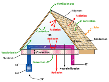 |
Figure 100. Vented attic thermal
processes. |
The importance of ceiling heat flux has long been recognized, with insulation a proven means of controlling excessive gains. However when ducts are present in the attic, the magnitude of heat gain to the thermal distribution system can be much greater than the ceiling heat flux. This influence may be exacerbated by the location of the air handler within the attic space - a common practice in much of the southern US. Typically an air handler is poorly insulated and has the greatest temperature difference at the evaporator of any location in the cooling system. It also has the greatest negative pressure just before the fan so that some leakage into the unit is inevitable.
The Flexible Roof Facility (FRF) is an FSEC test facility designed to evaluate five roofing systems at a time against a control roof with black shingles and vented attic (Figure 101). The testing evaluates how roofing systems impact summer residential cooling energy use and peak demand.
Final Year Experiments
The summer of 2005 featured the final reconfiguration of the test cells (Table 67) in FSEC’s Flexible Roof Facility (FRF). Test Cell #6 remained a white metal standing seam roof (best performer so far). Research will collect data on varied ventilation rates for FRF testing 2005 – a gap within the FSEC and roofing industry related research which is important to address. Instrumentation will obtain plywood decking moisture and attic moisture measurements as part of the protocol. All test cells were altered to R-30 insulation installed on the attic floor with the ventilation areas carefully verified by blower door pressurization. All test cells, except test cell #6, now have black shingle roofs. Relative humidity sensors are being used to evaluate how the different attic ventilation strategies influence attic moisture conditions.
Table 67. Roofing systems tested
at the
FSEC Flexible Roofing Facility, Summer of 2005
| Cell # | Description | Justification within experiment |
| 6 | White metal roof, 1:300 ventilation | Best performing roofing system |
| 5 | Reference, 1:300 ventilation area | Standard requirement for building codes |
| 4 | Black shingles, 1:150 vent area | Added attic ventilation area per codes |
| 3 | Black shingles, Sealed | New ASHRAE recommendation to reduce attic humidity |
| 2 | Black shingles, 1:300, soffit | Evaluate impact of soffit vs. ridge venting |
| 1 | Black shingles, 1:300, ridge | Evaluate impact of soffit vs. ridge venting |
Early research results show that the balance of the ridge vs. soffit ventilation is critical in the performance of added ventilation—solely ridge or soffit vents (Cells 1 and 3) are barely more effective than no ventilation at all. As expected, 1:150 ventilation is more thermally advantageous than 1:300 ventilation, but not by a large amount.
Tests were made by alternately opening and closing midway the ridge vents in Test cell #2 through the summer season to examine influences on performance. Relative humidity sensors were used to evaluate how the different attic ventilation strategies influence attic moisture conditions. Final analysis results will be published in the fall of 2006.
6th Budget Period Experiments
In the summer of 2004, the following roofing systems were tested (Table 68). Cell numbering is from left to right.
Table 68. Roofing systems tested at the FSEC
Flexible Roofing Facility, Summer of 2004
| Cell # | Description |
| 1 | Galvalume®* unfinished (unpainted) 5-vee metal with vented attic (3rd year of exposure) |
| 2 | Proprietary test cell |
| 3 | Proprietary test cell |
| 4 | Galvanized unfinished 5-vee metal with vented attic (3rd year of exposure) |
| 5 | Black shingles with standard attic ventilation (Control Test Cell) |
| 6 | White standing seam metal with vented attic (3rd year of exposure after cleaning) |
All had R-19 insulation installed on the attic floor. The measured thermal impacts include ceiling heat flux, unintended attic air leakage and duct heat gain. Test Cells #2 and #3 had proprietary test configurations that are not further described in this report.
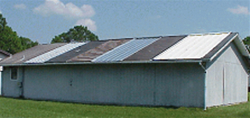 |
Figure 101. Flexible Roof Facility
in summer of 2003 configuration. |
The white metal roof results in the coolest attic over the summer, with an average day peak air temperature of only 95.7°F – 22.2° cooler than the peak in the control attic with dark shingles.
This was the third year of comparative testing metal roofing (galvanized and Galvalume®) under long term conditions. Galvalume® roofs are reported to better maintain their higher solar reflectance than galvanized types. Average daily mid-attic maximum temperatures for the Galvalume® and galvanized metal roof systems showed significantly better performance for Galvalume® product (10.9°F and 2.1°F cooler than the control dark shingle respectively). However, both unfinished metal roofs showed significant degradation in their performance over the three year period compared to the white metal roof.
We also estimated the combined impact of ceiling heat flux, duct heat gain and unintended attic air leakage from the various roof constructions. The alternative constructions produced lower estimated cooling energy loads than the standard vented attic with dark shingles. The Galvalume® roof clearly provided greater reductions to cooling energy use than the galvanized roof after three summers of exposure, although both suffered significant degradation relative to the first year’s performance. More specifically, the Galvalume® and Galvanized roof system provided a 32% and 22% savings in the first year of exposure, but only 12% and 1% respectively after three years of exposure.
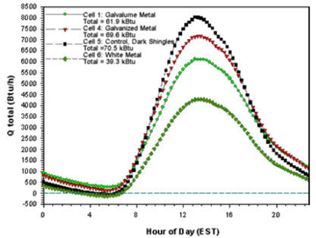
Figure 102. 2004 Results Estimated
combined impact of duct heat gain, air leakage
from the attic to conditioned
space and ceiling heat flux on space cooling needs
on an average summer day
in a 2,000 ft2 home.
One important fact from our testing is that nighttime attic temperature and reverse ceiling heat flux have a significant impact on the total daily heat gain, particularly for the metal roofs. The rank order below shows the percentage reduction of roof/attic related heat gain and approximate overall building cooling energy savings (which reflect the overall contribution of the roof/attic to total cooling needs):
Table 69. Cooling Load Reduction and Savings
| Rank | Description | Roof Cooling Load Reduction | Overall Cooling Savings |
| 1 | White Metal with vented attic (Cell #6) | 44% |
15% |
| 2 | Galvalume® unfinished metal with vented attic (Cell #1) | 12% |
4% |
| 3 | Galvanized unfinished metal roof with vented attic (Cell #4) | 1% |
0% |
The relative reductions are consistent with the whole-house testing recently completed for FPL in Ft. Myers (Parker et al., 2001). This testing showed white metal roofing having the largest reductions, followed by darker constructions. After long-term exposure, test results indicate that galvanized metal roofing is no better than a standard asphalt shingle roof after three years of exposure. On the other hand, the Galvalume roof does maintain some advantage although not nearly so great as the white metal type.
5th Budget Period Experiments
The roofing systems tested in the summer of 2003 are listed in Table 70. Cell numbering is from left to right beginning with the second cell in from the left.
Table 70. Roofing systems tested at the FSEC
Flexible Roofing Facility, Summer of 2003
| Cell # | Description | |
| 1 | Galvalume®* unfinished 5-vee metal with vented attic (2nd year of exposure) | |
| 2 | Sealed attic with proprietary configuration | |
| 3 | High reflectance brown metal shingle with vented attic | |
| 4 | Galvanized unfinished 5-vee metal with vented attic (2nd year of exposure) | |
| 5 | Black shingles with standard attic ventilation (Control Test Cell) | |
| 6 | Standing seam metal with vented attic (2nd year of exposure after cleaning) | |
| * Galvalume is a quality cold-rolled sheet to which is applied a highly corrosion-resistant hot-dip metallic coating consisting of 55% aluminum 43.4% zinc, and 1.6% silicon, nominal percentages by weight. This results in a sheet that offers the best protective features characteristic of aluminum and zinc: the barrier protection and long life of aluminum and the sacrificial or galvanic protection of zinc at cut or sheared edges. According to Bethlehem Steel, twenty-four years of actual outdoor exposure tests in a variety of atmospheric environments demonstrate that bare Galvalume sheet exhibits superior corrosion-resistance properties. | ||
All had R-19 insulation installed on the attic floor except in the configuration
with the sealed attic (Cell #2) which had R-19 of open cell foam sprayed onto
the bottom of the roof decking. The measured thermal impacts include ceiling
heat flux, unintended attic air leakage and duct heat gain. Cell #2 had a proprietary
configuration which is not reported upon in this report.
A major thrust of the testing for 2003 was comparative testing of metal roofing
under long term exposure. Given the popularity of unfinished metal roofs, we
tested both galvanized and Galvalume® roofs in their second year of exposure..
Average daily mid-attic maximum temperatures for the Galvalume® and galvanized
metal roof systems showed significantly better performance for Galvalume® product
(17.5oF and 13.1oF cooler than the control dark shingle respectively).
Other than the sealed attic case, the white metal roof results in the coolest attic over the summer, with an average peak of only 94.6oF – 22.1o cooler than the peak in the control attic with dark shingles. The highly reflective brown metal shingle roof (Cell #3) provided the next coolest peak attic temperature. Its average maximum daily mid-attic temperature was 101.5oF (15.2oF lower than the control dark shingle cell). While the brown metal shingle roof’s reflectance was lower than the two metal roofs and white metal roof we observed evidence that the air space under the metal shingles provides additional effective thermal insulation.
We also estimated the combined impact of ceiling heat flux, duct heat gain and unintended attic air leakage from the various roof constructions. All of the alternative constructions produced lower estimated cooling energy loads than the standard vented attic with dark shingles (Figure 103). The Galvalume® roof clearly provided greater reductions to cooling energy use than the galvanized roof after two summers of exposure.
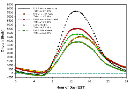
Figure 103. Estimated combined
impact of duct heat gain, air leakage
from the attic to conditioned space
and ceiling heat flux on space cooling
needs on an average summer day in
a 2,000 ft2 home.
Nighttime attic temperature and reverse ceiling heat flux have a significant impact on the total daily heat gain, particularly for the metal roofs. The rank order in Table 71 shows the percentage reduction of roof/attic related heat gain and approximate overall building cooling energy savings (which reflect the overall contribution of the roof/attic to total cooling needs):
Table 71. Roof cooling load reduction and
overall
cooling savings, Summer 2003
| Rank | Description | Roof Cooling Load Reduction |
Overall Cooling Savings |
| 1 | White metal with vented attic (Cell #6) | 47% |
15% |
| 2 | High reflectance brown metal shingle with vented attic (Cell #3) | 29% |
10% |
| 3 | Galvalume® unfinished metal with vented attic (Cell #1) | 25% |
8% |
| 4 | Galvanized unfinished metal roof with vented attic (Cell #4) | 16% |
5% |
4th Budget Period Experiments
In the summer of 2002, six roofing systems were evaluated as described in Table 72 and Figure 104.
Table 72. Roofing systems tested and associated
energy savings at
the FSEC Flexible Roofing Facility, Summer of 2002
| Cell # | Roof Material | Venti- lation |
Roof Cooling Load Reduction |
Overall Cooling Savings |
| #1 | Galvalume® unfinished 5-vee metal | vented |
32% |
11% |
| #2 | double roof with radiant barrier (ins roof deck) | sealed |
7% |
2% |
| #3 | high reflectance ivory metal shingle | vented |
38% |
12% |
| #4 | galvanized unfinished 5-vee metal | vented |
22% |
7% |
| #5 | black shingles (control cell) | vented |
control |
control |
| #6 | white standing seam metal | vented |
7% |
2% |
All roof cells had R-19 insulation installed on the attic floor, except the double roof configuration (Cell #2) which had a level of R-19 open cell foam sprayed onto the bottom of the roof decking. Measured thermal impacts included ceiling heat flux, unintended attic air leakage, and duct heat gain.
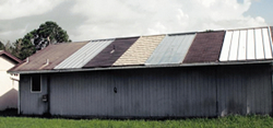 |
Figure 104. Flexible Roof Facility
in summer 2002 configuration. Cells are numbered from left to right starting
with the second cell in from the left. |
The sealed attic double roof system (Cell #2) provided the coolest attic space of all systems tested (average maximum mid-attic temperature was 81.1oF), and therefore had the lowest estimated impact due to return air leakage and duct conduction heat gains. However this cell also had the highest ceiling heat flux of all strategies tested, and recorded the most modest space cooling reduction (7%), relative to the control roof.
Metal roof testing was given more emphasis in 2002 due to the popularity of
these products. Researchers tested both galvanized and Galvalume® roofs.
Galvalume is a cold-rolled sheet with a highly corrosion-resistant hot-dip
metallic coating application of 55% aluminum 43.4% zinc, and 1.6% silicon.
These roofs are reported to better maintain solar reflectance than galvanized
roofing systems. Average daily mid-attic maximum temperatures for the Galvalume® and
galvanized metal roof systems were roughly similar (19.6oF and 17.3oF cooler
than the control roof, respectively). The estimated total heat gain for these
roof cells also was relatively close.
The highly reflective ivory metal shingle roof (Cell #3) provided the coolest
peak attic temperature of all the cells without roof deck insulation. Its average
maximum daily mid-attic temperature was 93.3oF (23.4oF lower than the control
dark shingle cell). While the ivory metal shingle roof’s reflectance
was slightly lower than the two metal roofs and white metal roof, researchers
noted that the air space under the metal shingles provided additional effective
thermal insulation.
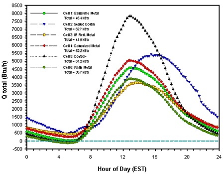
Figure 105. 2002 estimated
combined impact of duct heat gain, air
leakage from the attic to conditioned
space, and ceiling heat flux on
space cooling needs on an average summer
day in a 2,000 ft2 home.
Researchers also estimated the combined impact of ceiling heat flux, duct heat gain, and unintended attic air leakage from the various roof constructions. All of the alternative roofing treatments produced lower estimated cooling energy loads than the standard vented attic with dark shingles. (Figure 105) The Galvalume® roof clearly provided a greater cooling energy use reduction than the galvanized roof. This also was true during the 2001 study. Nighttime attic temperatures and reverse ceiling heat flux have a significant impact on the total daily heat gain, particularly for metal roofs.
3rd Budget Period
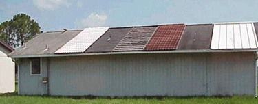 |
Figure 106. 2001 Experimental
roof cell. Cells are numbered from left to right starting with the cell second in from the left. |
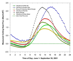
In the 2001 testing, Cell #2 with the double roof/sealed attic showed the lowest attic temperatures and narrowest temperature range. (Table 73; Figures 107 and 108) Peak attic temperatures in Cell #2 were 5oF to 6oF lower than this same sealed cell the year before, without the double roof. This indicates that the double roof did provide a substantial benefit. Since there is no insulation on the attic floor though, there still is a significant heat gain across the ceiling. In fact, the ceiling heat fluctuation actually is higher than the reference Cell #5. (Figure 107)
 |
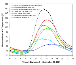 |
Figure 107. (left) 2001 heat flux measurements across attic. |
Figure 108. (right) 2001 mid-attic temperatures. |
The true impact of the double roof construction of Cell #2 is most likely
a combination of the benefits of a cooler attic space that reduces duct heat
gain and minimizes the effects of air leakage from the attic into the house,
and the drawback of the higher ceiling heat flux.
Cell #3 with its spectrally selective dark brown metal shingles, produced lower
attic temperatures at night, but higher roof deck temperatures (which were
most likely due to the insulating quality of the shingles which have an air
space underneath them).
Table 73. Roofing systems tested and
attic temperatures at
the FSEC Flexible Roofing Facility, Summer of 2001
| Cell # | Roof Material | Venti- lation |
Avg Attic Temp |
Max Attic Temp |
| #1 | white tile (weathered) | sealed |
84.6 |
111.2 |
| #2 | double roof with radiant barrier (ins roof deck) | sealed |
78.4 |
85.4 |
| #3 | brown IR selective metal shingle | vented |
85.0 |
110.8 |
| #4 | terra cotta tile (weathered) | vented |
89.0 |
124.3 |
| #5 | dark shingles (control) | vented |
91.0 |
143.4 |
| #6 | white standing seam metal (weathered) | sealed |
84.0 |
115.5 |
Roofing Experiment with Habitat for Humanity in Fort Myers, Florida
In July 2000, FSEC and Florida Power and Light instrumented six side-by-side Habitat for Humanity homes in Ft. Myers with identical floor plans, orientation, and ceiling insulation, but with different roofing systems as described in Table 74. A seventh monitored house contained an unvented attic with insulation on the underside of the roof deck rather than on the ceiling.
Each unoccupied home was monitored from July 8 through July 31, 2001 to collect building thermal and air conditioning power data. Table 75 presents the cooling performance of the roofing systems clearly showing the energy-saving benefits of reflective roofing systems in Florida, especially the tile and metal roofs with solar reflectance between 65% and 75%.
Table 74. Roofing systems tested at side-by-side
Habitat for Humanity homes in Ft. Myers Summer of 2000
| Code | Description | Code | Description |
| RGS | Standard dark shingles (control) | RTB | Terra cotta "barrel" S-tile roof |
| RWS | Light colored shingles | RWB | White "barrel" S-tile roof |
| RWM | White metal roof | RWF | White flat tile roof |
| RSL | Standard dark shingles with sealed attic & R-19 roof deck insulation |
Table 75. Energy use and savings from roofing
systems in
Habitat for Humanity roofing study, summer of 2000
Site |
Total kWh |
Savings kWh |
Saved Percent |
Demand kW |
Savings kW |
Saved Percent |
RGS |
17.03 |
---- |
---- |
1.63 |
---- |
---- |
RWS |
15.29 |
1.74 |
10.2% |
1.44 |
0.19 |
11.80% |
RSL |
14.73 |
2.30 |
13.05% |
1.63 |
0.01 |
0.30% |
RTB |
16.02 |
1.01 |
5.9% |
1.57 |
0.06 |
3.70% |
RWB |
13.32 |
3.71 |
21.8% |
1.07 |
0.56 |
34.20% |
RWF |
13.20 |
3.83 |
22.5% |
1.02 |
0.61 |
37.50% |
RWM |
12.03 |
5.00 |
29.4% |
0.98 |
0.65 |
39.70% |
Significant findings: Reflective roofing materials represent one of the most significant energy-saving options available to homeowners and builders. These materials also reduce cooling demand during utility coincident peak periods, and are potentially one of the most effective methods for controlling demand.
Research by BAIHP Researcher Neil Moyer with BAIHP Industry Partner Tamarack
Scope
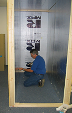 |
Figure 107. Return
Air Flow Test Chamber |
In effect since March 2003, Section 601.4 of the Florida Building Code applies to residential and commercial buildings having interior doors and one, centrally located return air intake per heating and cooling system.
Objective Of The New Florida HVAC Code Requirement
Reduce pressure difference in closed rooms with respect to (wrt) the space where the central return is located to 0.01” water column (wc) or 2.5 Pascal (Pa) or less. Pressure imbalances created by restricted return air flow from rooms isolated from the central return by closed interior doors create uncontrolled air flow patterns.
Technical Background
Ideally, forced-air heating and cooling systems circulate an equal volume of return air and supply air through the conditioning system, keeping air pressure throughout the building neutral. Each conditioned space in the building should, ideally, be at neutral air pressure at all times.
When a space is under a positive air pressure, indoor air will be pushed outward in the walls, floor and ceiling. When a space is under a negative pressure, air will be pulled inward through the walls, floor and ceiling. Negative and positive air pressures in buildings result from uncontrolled air flow patterns.
Section 601.4 of the Florida Building Code specifically deals with the uncontrolled air flow pattern when interior doors are closed thereby reducing return air flow from the closed room, while maintaining the same supply air flow to the room. This imbalance of supply and return air has been addressed conventionally by the common practice of undercutting interior doors to allow return air to flow from the room. This research quantifies the volume of air flow provided by this and other methods of return air egress from closed rooms.
Section 601.4 limits the air pressure imbalance in closed rooms to 0.01” wc or 2.5 pascals when compared to, or with respect to (wrt), the main body of the building where the return is located. With door undercuts, researchers have regularly observed room pressures with respect to the main body of the house (wrtmainbody) of +7 pascals (pa) or more. A room with this level of air pressure (+7pa, wrtmainbody) is trapping air, starving the heating/cooling system of return air. As the heating/cooling system struggles to pull in the designed amount of air, the resulting negative pressure pulls air into the main body of the building along the path(s) of least resistance. Usually this means that air is flowing through the walls, floor and ceiling from unconditioned spaces or outside environment to makeup for the trapped air in the closed room.
In the closed room, positive pressure builds up when return air is trapped. Conversely, the space with the central return gets depressurized because extra return air is being removed to make up for the air trapped in the closed room. More air is leaving the space (return air) than is entering the space (supply air). The positive pressure in the closed rooms pushes air into unconditioned spaces, such as the attic and wall cavities. The negative pressure in the main body of the building pulls air from unconditioned spaces. In Florida, the air brings heat and moisture with it that becomes an extra cooling load. This air is referred to as “mechanically induced infiltration” since the negative pressure drawing infiltration air in was created by the mechanical system.
Styles of Pressure Relief
When return air flow is restricted by closed doors, it creates pressure differences between parts of the building. This can be prevented by installing a fully ducted return system, by creating a passive return air pathway such as a louvered transoms, door undercut, “jump duct”, through-wall grilles, or a baffled through-wall grill.
A “jump duct” is simply a piece of flex duct attached to a ceiling register in the closed room and another ceiling register in the main body of the house. A jumper duct provides some noise control while providing a clear air flow path.
A through-wall grille is the simplest and least expensive approach to pressure relief for closed rooms. Holes opposite each other on either side of the wall within the same stud bay are covered with a return air grilles. The downside of this approach is a severe compromise the privacy of the closed room. An improvement on this theme would be to locate one of the grilles high on the wall and the opposing opening low on the wall. Also, such openings in interior wall cavities introduce conditioned air into what is typically an unconditioned space possibly contributing to other building problems.
However, connecting the two openings with a sleeve of rigid ducting forms an enclosed air flow path that limits introduction of conditioned air into the wall cavity but doesn’t solve the visual and sound privacy issues. To address this problem, BAIHP Industry Partner Tamarack developed a sleeve with a baffle that can reduce the transfer of light and sound but still provide adequate air flow to minimize pressure differences. The product is called a Return Air Path (RAP).
To validate the effectiveness of this product and other approaches to providing return air pathways, Tamarack and BAIHP researchers devised a test apparatus and conducted experiments in FSEC’s Building Science Laboratory.
Testing Protocol
In May of 2003, a chamber was constructed at FSEC (Figures 107-110) that simulated a frame construction room with an 8 foot high ceiling. A “Minneapolis Duct Blaster” was connected to one end of the room with a flexible duct connection leading out of the room to provide control over pressure in test chamber.
In the middle of the chamber, on a stool, a radio was tuned “off station” to effectively create a standardized level of “white noise” at 57 dBA inside the chamber with the “door” closed. The temperature at the start of the tests was 80°F at 40%RH. A sound meter was located outside the chamber on a stand 4 feet above the floor and 20 inches from the middle of the chamber wall surface.
The sound level in the test facility outside the chamber with the “white noise” turned off was 36.4 dBA and with the “white noise” turned on was 41.5 dBA, an average, sampled over a 30 second period. A series of tests on 31 different set-ups were performed, measuring the flow at 3 different pressure levels and recording a 30 second sound sample with the “Duct Blaster” deactivated.
Tests were made for 6” and 8” jump ducts, five different sized wall openings (Figure 107) in different configurations including straight through with and without sleeves, straight through with sleeve and privacy baffle (Figure 108), and high/low offset using the wall cavity as a duct, and three different slots simulating three different size undercut doors.
Results
Table 76 summarizes the results of these tests arranged in ascending air flow order based on the results at 2.5 Pascals (0.01” wc), the maximum allowable pressure in a closed room under new requirement in Florida Building Code, Section 601.4.
 |
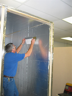 |
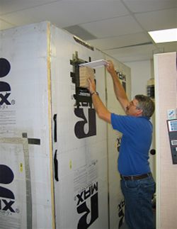
Figure 108. Installing
sound baffled return air flow through wall insert made by Tamarack. |
Figure109. Installing unbaffled return air flow through wall grille |
Table 76. Air Flow Resulting from Various Return Air
Path Configurations
at Controlled Room Pressure Difference
(ΔP) with respect to Return
Zone
Dim. |
Air
Flow (cfm) at |
Area |
Air
Flow to Area Ratio |
Return
Air Path Configuration |
Extra |
||
ΔP=1
pa |
ΔP=2.5 pa |
ΔP=5
pa |
|||||
6 dia |
22 |
36 |
52 |
28 |
1.29 |
Jumper Duct |
|
4x12 |
26 |
41 |
60 |
48 |
0.85 |
Wall Cavity |
|
4x12 |
25 |
42 |
61 |
48 |
0.88 |
Wall Sleeve |
RAP Insert |
4x12 |
28 |
45 |
65 |
48 |
0.94 |
No Sleeve |
|
4x12 |
29 |
46 |
68 |
48 |
0.96 |
Wall Sleeve |
|
8x8 |
31 |
49 |
72 |
64 |
0.77 |
Wall Cavity |
|
12x6 |
32 |
52 |
75 |
72 |
0.72 |
Wall Cavity |
|
12x6 |
33 |
56 |
82 |
72 |
0.78 |
Wall Sleeve |
RAP Insert |
8x8 |
35 |
57 |
81 |
64 |
0.89 |
No Sleeve |
|
8x8 |
34 |
58 |
83 |
64 |
0.91 |
Wall Sleeve |
RAP Insert |
8x8 |
36 |
59 |
85 |
64 |
0.92 |
Wall Sleeve |
|
12x6 |
36 |
60 |
88 |
72 |
0.83 |
No Sleeve |
|
12x6 |
37 |
60 |
88 |
72 |
0.83 |
Wall Sleeve |
|
1 x 30 |
39 |
61 |
88 |
30 |
2.03 |
Slot |
|
8 dia |
38 |
62 |
90 |
50 |
1.24 |
Jumper Duct |
|
1 x 32 |
42 |
65 |
92 |
32 |
2.03 |
Slot |
|
8x8 |
40 |
67 |
95 |
64 |
1.05 |
Wall Cavity |
Two Inside Holes |
8x14 |
44 |
70 |
100 |
112 |
0.63 |
Wall Cavity |
|
12x12 |
45 |
72 |
103 |
144 |
0.50 |
Wall Cavity |
|
1 x 36 |
49 |
73 |
103 |
36 |
2.03 |
Slot |
|
8x14 |
61 |
101 |
146 |
112 |
0.90 |
Wall Sleeve |
RAP Insert |
8x14 |
68 |
107 |
153 |
112 |
0.96 |
No Sleeve |
|
8x14 |
68 |
110 |
154 |
112 |
0.98 |
Wall Sleeve |
|
12x12 |
75 |
119 |
170 |
144 |
0.83 |
No Sleeve |
|
12x12 |
74 |
120 |
169 |
144 |
0.83 |
Wall Sleeve |
|
12x12 |
74 |
120 |
174 |
144 |
0.83 |
Wall Sleeve |
RAP Insert |
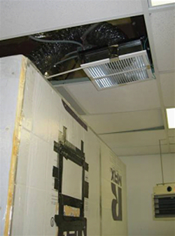 |
Figure 110. Return air flow path provided
by jumper duct |
By comparing the air flow of the slots (door undercut) to the openings with
grilles, the detrimental effect of the grille becomes clear. The ratio of air
flow (cfm) to the surface area of the slot (in2) is more than 2 to 1 (for example;
30 in2 to 61 cfm), whereas with grilles in place the ratio of air flow to area
averages 0.83 to 1 (for example; 72 in2 to 60 cfm). Similarly, the jump duct (Figure
110) assemblies’ air flow to area ratios average 1.19 to 1. In any
calculation for the size of the through wall assembly, the resistance of the
grille becomes the critical factor in determining the size of the opening for
achieving the desired flow.
The following formulas account for the grille resistance and maybe used to
size return air path openings.
Although there does not appear to be significant flow improvement when a sleeve is used, such an assembly will reduce the possibility of inadvertent air flow from the wall cavity itself.
The high/low grilles using the wall cavity reach maximum flow at 72 cfm because of the dimensional limitations of the wall cavity itself. Increasing the opening of each grille beyond 112 square inches does not significantly increase the flow of air through the wall cavity.
The accompanying bar chart (Figure 111) can be used to select the best method at various air flows while maintaining the room-to-building pressure difference at .01” wc. The strategies are ranked by air flow allowance (cfm) on equivalent to supply air delivered to the room. For example, an 8” jumper duct could be used to maintain 0.01 wc in rooms with supply air up to 60 cfm. Note that these transfer methods are additive so that, for example, combining a 6” transfer duct with a 1” undercut a 30” door, will provide a flow of 95 cfm to be delivered at .01” wc (Figure 99) or combining a R.A.P. 12.12 with a 1” undercut would allow up to 175 cfm to be delivered . It should be noted that door undercuts are under builder not HVAC control and that the actual dimensions are greatly affected by the thickness of the floor coverings.
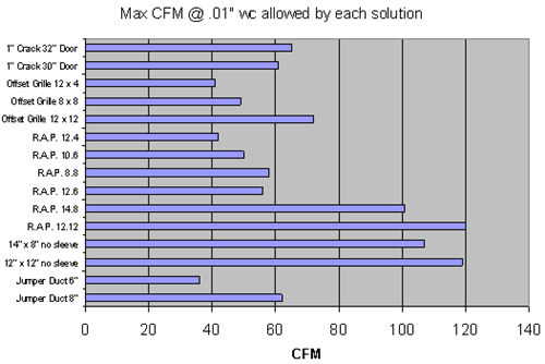
Figure 111. Maximum air flow achievable
using various return air paths from closed rooms for a
give supply at a room
pressure of 2.5 pa or 0.1” wc with respect to the return zone. For
example,
an 8” jumper duct could be used to maintain 0.01 wc in rooms
with supply air up to 60 cfm.
Summary
Ideally buildings with forced air heating/cooling systems are pressure neutral. The same amount of air is removed from the building (and each room) as is supplied to it. However, this balance can be disturbed in homes that have one, centrally located return intake when interior doors are closed, blocking return of air supplied to private rooms. Other factors outside the scope of this study may also result in household pressure imbalances.
These research results are relevant to homes with forced air heating and cooling systems having a single, centrally located return air inlet with no engineered path for return air to exit closed rooms. Such systems pull return air from the whole house as long as interior doors are open. When an interior door is closed, more air is supplied to the closed room than can be removed, or returned, from the room.
Positive pressure builds up in the closed room while a negative pressure occurs in the connected spaces. Positive pressure presses outward on all surfaces and may eventually reduce supply air flow into the closed room and while pushing conditioned air through small breaks in the room’s air barrier.
To overcome house pressure imbalances caused by door closure, a variety of passive return path strategies are studied including a product produced by BAIHP Industry Partner Tamarack that overcomes privacy issues associated with through-wall grills. Achievable air flows for jump ducts, through-wall grilles, sleeved through-wall grilles, and the Tamarack baffled through-wall grille are presented.
Research by BAIHP Researcher Carlos Colon
BAIHP researcher tested the efficiency of a heat pump water heater manufactured by EMI, a division of ECR International. The unit features a compressor (R-134A refrigerant) with a wrap-around heat exchanger mounted on top of a 50-gallon storage tank. The latest controller board model #AK 4001 was installed during the test.
The temperature regulation of the unit is achieved by an adjustable potentiometer which sets a resistance that is measured by the controller board and translated into the corresponding temperatures. The set temperature is stored in the controller’s memory.
The controller logic is designed to operate the heat pump when the temperature in the bottom of the tank drops below the effective dead band temperature of 30°F (20°F dead band + assumed stratification of 10°F). The heat pump shuts off when the temperature in the bottom of the tank has reached 10°F below the set point temperature. The upper element of the tank operates only when the temperature in the upper tank reaches 27°F below the set point temperature.
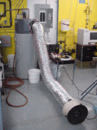 |
Figure 112. Airflow measurements
using a Duct tester on heat pump cold air discharge side. |
During laboratory testing the controller’s performance was evaluated by measuring inlet and outlet water temperatures using thermocouples mounted to the copper inlet and outlet pipes as well as a Fluke hand-held thermometer inserted into the hot water outlet stream. One minute average measurements during draws were in agreement with the 10°F stratification logic utilized by EMI.
Also, following a series of hot water draws during the efficiency test (described below), the compressed refrigerant heat was able to replenish the tank to the 130 °F temperature level. However, following the heating recovery, neither compressor or resistance element were activated during standby until three days later when bottom tank temperatures dropped below 95°F. The compressor was called into operation when the tank was submitted to a hot water draw which triggered the ON compressor event in less than a minute.
Table 77 is a summary of electrical efficiency results generated from three tests performed in the laboratory. Tank pre-heating for test #1 and #2 were performed in a similar way, by forcing the compressor to turn “ON”. The tank was allowed to loose heat on standby (1-2 days) and then purged with a draw of at least 30 gallons of new water. The purge forced the compressor to operate. Preheating for the test #3 was performed with the tank relatively hot and only twelve gallons of hot water were purged. This might explain the higher outlet temperatures read during test 3. For all three tests, we attempted to heat water so that initial hot water draws were near 130 °F (+/- 5 °F). However, we noticed that temperatures at the top of the tank (upper level) increased slightly with each purge (i.e., 10.7 gallon draw). During the third test shown in Table 61 for example, outlet temperatures during the first draw averaged 129.2 °F, but during the last draw temperatures reached an average of 143.4 °F. The values for test #3 show an overall hot water delivery temperature (Toutlet) of 136.6 °F. The controller never called for compressor or auxiliary energy when left on standby during the completion of the test (24-hr.).
Table 77. Electrical Efficiency Results from Laboratory Tests
| Test | Total Gallons Drawn |
Average Tinlet (°F) |
Average Toutlet
(°F) |
Total Qout kWh |
Total Qin kWh |
COP |
| #1 | 63 |
82.3 °F |
133.2 °F |
7.756 |
3.974 |
1.95 |
| #2 | 53.5 |
82.1 °F |
131.2 °F |
6.533 |
3.516 |
1.86 |
| #3 | 65.9 |
82.0 °F |
136.4 °F |
8.789 |
4.254 |
2.06 |
Conclusions
The WattSaver™ heat pump water heater is rated with an energy factor (EF) of 2.45 and clearly demonstrates that heating water can be accomplished at a relative higher efficiency when compared to conventional electric water heaters. Installed in a conditioned space, and under operation with inlet water temperatures above 80 °F (e.g., Central Florida summer water mains temperatures), an average electrical (COP) efficiency of 2.0 was attained. Other measurements and performance indicators are summarized in Table 78.
Table 78. Summary of Other Measurements and Performance Overview
| Typical Cooling Air Flow rate: 87 CFM (Figure 87) Top cavity/Fan operating : -6.4 pa Evaporator Air temp: 73 °F (63%RH entering) / 53.1 °F (leaving) Condensate: 502.6 g/hr. (1.1 lb/hr) Sensible: 1900 Btu/hr. Latent: 957 Btu/hr Total Capacity : 2,857 Btu/hr |
Current consumption (208 VAC) Compressor2.9 amps Fans (2) : 0.08 Amps/each Total 3.08 amps |
Two caveats to the heat pump water heater’s performance was first the delayed recovery during standby which would present larger hot water temperature variation to the residential user. This also leads to diminished hot water capacity during long periods of no hot water use activity. Second, because the compressor’s discharge refrigerant (i.e., hottest temperatures) enter the wrap-around heat exchanger at the top of the tank, the unit demonstrated larger hot temperature variations at the tank’s upper levels when the top portion was all pre-heated. These stratified tank temperature levels differ from those obtained when heating is started with the tank filled up with mains (colder) water conditions.
Study led by BAIHP Researcher Danny Parker
Papers: Parker, D. S.. "Theoretical Evaluation of the NightCool Nocturnal Radiation Cooling Concept". Submitted to: U.S. Department of Energy. FSEC-CR-1502-05. April 2005.
Parker, Danny S. and John R. Sherwin, 2006. “Experimental Evaluation of the NightCool Nocturnal Radiation Cooling Concept: Progress Report: Initial Thermal Performance Assessment of Test Buildings. FSEC-CR-1657-06, Florida Solar Energy Center, Cocoa, Florida. September 2006.
Technical Background
Using a building’s roof to take advantage of long-wave radiation to the night sky has been long identified as a potentially productive means to reduce space cooling in buildings. This is because a typical roof at 75° F will radiate at about 55-60 W/m2 to clear night sky and about 25 W/m2 to a cloudy sky. For a typical roof (250 square meters), this represents a cooling potential of 6,000 - 14,000 Watts or about 1.5 - 4.0 tons of cooling potential each summer night. Various physical characteristics (differential approach temperature, fan power, convection and conductance) limit what can be actually achieved, so that perhaps half of this rate of cooling can be practically obtained. Even so, careful examination of vapor compression space cooling in many homes in Florida shows that typical homes experience cooling loads averaging 33 kWh per day from June - September with roughly 9.2 kWh (28%) of this air conditioning coming between the hours of 9 PM and 7 AM when night sky radiation could greatly reduce space cooling.
A big problem with night sky radiation cooling concepts has been that they have typically required exotic building configurations. These have included very expensive “roof ponds” or, at the very least, movable roof insulation with massive roofs so that heat is not gained during daytime hours. The key element of our new configuration is that rather than using movable insulation with a massive roof or roof ponds, the insulation is installed conventionally on the ceiling. The operation of the system is detailed in the attached schematic.
During the day, the building is de-coupled from the roof and heat gain to the attic space is minimized by a white reflective metal roof. During this time the space is conventionally cooled with a small air conditioner. However, at night as the interior surface of the metal roof in the attic space falls two degrees below the desired interior thermostat set point, the return air for the air conditioner is channeled through the attic space by way of electrically controlled louvers with the variable speed. The warm air from the interior then goes to the attic and warms the interior side of the metal roof which then radiates the heat away to the night sky. As increased cooling is required, the air handler fan speed is increased. If the interior air temperature does not cool sufficiently or the relative humidity is not kept within bounds (<55% RH) the compressor is energized to supplement the sky radiation cooling. A dehumidifier is used when temperature conditions are favorable, but moisture conditions are not. The massive construction of the building interior (tile floor and concrete interior walls) will store sensible cooling to reduce space conditioning needs during the following day.
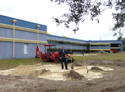 |
Figure 113. Groundbreaking for the Nightcool
instrumented experimental buildings, Florida Solar Energy Center |
Experimental Design
To verify the potential of the concept, the radiative cooling system will be
tested in two 10 x 16' test structures. These highly instrumented buildings
are located just south of the Building Science Lab (Figure 113) at
the Florida Solar Energy Center (FSEC). Design and siting issues were resolved
in 2004, and construction began in 2005.
One of the test sheds will be the control structure with a standard attic with
R-19 ceiling insulation and an asphalt shingle roof with 1:300 ventilation
rate. The experimental unit will have a white metal roof on metal battens and
a sealed attic, which can be convectively linked to the main zone by a powered
circulation fan. Both units will have slab floors, frame walls and solar control
small double glazed windows.
A schematic of the test case and a similar drawing of the concept in a real home are shown in Figures 115 and 116.
6th Budget Period: Detailed Simulation Model
During the 6th budget period a detailed simulation model was created. Once the simulation model was validated against known solutions (Givoni, 1994 and Santamouris and Asimakopolous, 1996), the model was then mated to TMY2 hourly weather data to predict performance around the year under realistically changing weather conditions. For the calculations we use Tampa, Florida TMY2 data adjusting the weather data wind speed to account for the greatly diminished velocity seen over roof tops in experiments done at the Flexible Roof Facility (Parker and Sherwin, 1998). Florida weather is less advantageous for the analysis than many other locations since high summer dew points will often limit cooling potential. However, this allows evaluation of the concept under difficult environmental conditions
The seasonal analysis for Tampa from June - September showed that the nocturnal system would operate an average of 8.6 hours per day, producing an average of 15.2 kWh of cooling per day for a home with a consumption of fan energy of 1.4 kWh. In a typical Florida house using 33 kWh/day this could offset about 46% of required space cooling if all could be effectively utilized. The system average operating energy efficiency ratio (EER) was 37.1 compared too 10-15 for common vapor compression air conditioners. The average daily profile of performance is shown in Figure 103 which shows the system performance.
Simulation in Other Climates
To examine concept performance elsewhere, we conducted the same simulation
in three additional climates which we expected to evidence substantially different
potentials. These were Atlanta, Georgia, reflecting a more moderate cooling
dominated climate, Baltimore, Maryland with a mixed heating and cooling climate
and Phoenix, Arizona with an arid, very hot climate.
Results are shown in Table 79. For comparison, performance indicated
from the simulation for June - September are provided alongside those for Tampa,
Florida. We also provide the results for the month of July in parentheses to
illustrate how the cooling potential varies during the hottest conditions in
each location.
Table 79. NightCool
Simulation Results for Other Climates
June - September and (July Only)
Parameter |
Tampa, FL |
Atlanta, GA |
Baltimore, MD |
Phoenix, AZ |
Avg Daily Cooling kWh Avg Hrs per Night Fan kWh COP SEER (Btu/Whr) |
15.2 (10.8) 8.6 (7.6) 1.4 (1.3) 10.9 (8.3) 37.1 (28.4) |
50.3 (42.4) 14.3 (13.9) 2.4 (2.3) 21.0 (18.4) 71.5 (62.9) |
62.4 (45.4) 14.6 (13.6) 2.4 (2.3) 26.0 (19.7) 88.7 (67.4) |
23.2 (11.2) 7.9 (5.3) 1.3 (0.9) 17.8 (12.4) 60.9 (42.5) |
Note that each climate other than Tampa shows better performance for the concept, both in absolute cooling and in overall cooling efficiency. Atlanta and Baltimore clearly indicate the concept to produce more cooling during evening hours than could be effectively utilized. For these locations, this would suggest both interior thermal storage and nighttime dehumidification to further offset daytime cooling needs.
The very hot climate of Phoenix, however, shows that like Tampa, the concept would only be able to offset 20 - 30% of daily cooling needs, although seemingly with the potential to essentially eliminate air conditioning loads during the swing months of April - May and October. Although Phoenix has less cloud cover, and greater diurnal temperature swing, the ambient evening temperatures tend to be hotter. Consequently, in this location, the NightCool system often does not start operation until after midnight. Even so, the concept showed efficient operation in all climates along with substantial ability to offset cooling needs in more temperate locations.
Progress during the Final Year of the Project
A contract report on theoretical performance was completed in April 2005 and placed online: "Theoretical Evaluation of the NightCool Nocturnal Radiation Cooling Concept". Submitted to: U.S. Department of Energy. FSEC-CR-1502-05. This report has garnered considerable interest. Parker presented data on the evaluation of the NightCool concept at the World Energy Sustainable Energy Conference in Wels, Austria on 1 March 2006. There was considerable international interest in the concept given the number of metal roofs in northern Europe. (Travel expenses were covered by non-BAIHP sources)
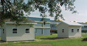 |
Figure 114. NightCool buildings at
FSEC |
Both the control building and experimental buildings were completed and the empirical evaluation of the concept is in progress. The control unit is configured like a conventional home with a dark shingle roof and insulated ceiling under a ventilated attic. The experimental unit features a white reflective roof on battens with a sealed attic where the air from the shed interior can be circulated to the sealed attic and roof radiator when the roof temperature drops well below the room target cooling temperature. A second contract report in September 2006 provides a brief evaluation of the performance of NightCool under static conditions with no mechanical cooling. Two experimental configurations were evaluated:
The experiments shows that NightCool performed better thermally under both configurations. With the NightCool linkage to the main zone disabled the average nighttime temperatures in the unconditioned experimental and control test buildings from 8 PM to 8 AM was 82.0 and 82.6°F respectively. This shows the experimental buildings runs slightly cooler at night, largely because of the lower attic temperatures across the insulation and the effectiveness of the R-30 SIPs panels in the ceiling against the R-30 fiberglass batts in the control.
However, in the second configuration with an attic hatch opened to the attic to allow warm air to naturally convect into the attic and heavier cool air to naturally convect to the interior below, the NightCool building showed superior performance. The experimental building’s interior ran 1.9°F cooler during nighttime hours without any mechanical air movement to aid heat transfer– this is about three times the temperature drop seen without any nighttime cooling. A good demonstration of nocturnal cooling within the concept.
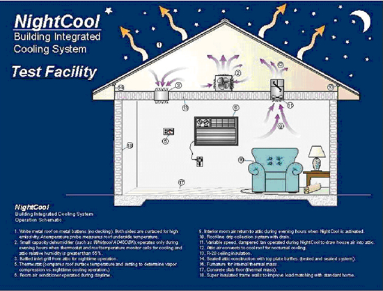
Figure 115. -Scehmatic design for NightCool test facility.
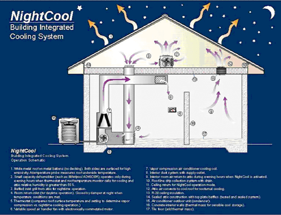
Figure 116. Schematic of NightCool concept in typical residential building.
Plug Load Reduction Study
Central Florida
Papers: Parker, D., Hoak, D., Meier,
A., Brown, R., "How Much Energy Are We Using? Potential of Residential
Energy Demand Feedback Devices", Proceedings of the 2006 Summer Study
on Energy Efficiency in Buildings, American Council for an Energy Efficient
Economy, Asilomar, CA., August 2006.
Richard Brown, William Rittelmann, Danny Parker, and Gregory Homan. Appliances, Lighting, Electronics, and Miscellaneous Equipment Electricity Use in New Homes Proceedings of the 2006 Summer Study on Energy Efficiency in Buildings, American Council for an Energy Efficient Economy, Asilomar, CA., August 2006
In the final year of the project, BAIHP began investigations into plug loads. This aspect of home energy use is changing rapidly with the constant expansion of the home electronics industry. To achieve DOE’s long range 70% energy saving goal, researchers will need to address control strategies and plug load management. Since occupant life style dictates this area of energy use, control strategies will need to be user friendly with simple readouts and operating instructions.
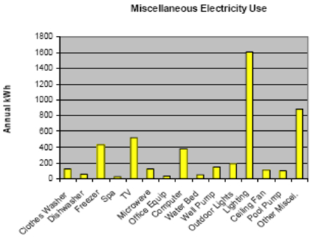
Figure 117. Plug load energy use
profile developed from data collected using commercially
available residential
feedback monitor and an FSEC developed audit protocol.
Before development of control systems, researchers need a clearer understanding of the energy use profile of plug loads BAIHP began to characterize plug loads by installing commercially available residential energy feedback monitors in five homes. Researchers developed an audit protocol which was successfully conducted in each home (Figure 117). Demonstrated savings of 2 kWh/day using simple switches and controls in one home through using the protocol with the feedback device to understand which devices were using power when appearing to be “off.” Switchable power strips reduced “off” loads. Coordinating effort with Rich Brown and Alan Meier at LBNL.
Solar Integrated Roofing Panels
Stuart, Florida
In the final year of the project, design assistance was provided to Nat Schwartz of NatMax for solar systems to be installed on the proposed homes in Coral Gables, Florida. Options presented included building integrated photovoltaic (BIPV) metal or tile systems. Technical assistance was provided during conference calls with Steven Crimi regarding the construction of new homes using SIP construction. Mr. Crimi is very interested in developing a new technique for BIPV in SIP construction. The concept would be evaluated side-by-side with currently available BIPV products to compare performance, ease of construction, cost, and aesthetics.
Hot Water Distribution Systems Research
During the final year of the project, researchers conducted a literature search on the topic of hot water distribution and re-circulation systems for residential/commercial buildings including magazine articles, professional papers, presentation files, independent roadmap plan strategies, and documents from the California Energy Commission’s (CEC) 2005 Building Energy Efficiency Standards and Action Items for the 2008 Standards on Hot Water Distribution Systems These two CEC documents analyze distribution loss sensitivity to floor area and number of stories, including parallel, trunk-branch distribution systems and hot water re-circulation strategies.
Researchers began further investigation of the current advances in hot water distribution models from Davis Energy Group (DEG - HWSIM), Oak Ridge National Laboratory Model (Synergistic Water Heating Technology PIER program) and NREL - NAHB using TRNSYS to assess the strengths, weaknesses, and development needs of each model.
Building America Benchmark Toolkit
for Programmers
Paper: Vieira, R., L. Gu, S. Se, C. Colon
(2006.) "Improving the Accuracy and Speed for Building America
Benchmarking." Florida Solar Energy Center, FSEC-CR-1651-R00, Aug. 29,
2006
The Building America Benchmarking process is time consuming. No simulation software currently is available to automatically generate the Bench mark version of the prototype home. Thus, analysts must first enter the parameters of the prototype home design into the Building America Benchmark Spreadsheet tool to create the parameters of the Building America benchmark home and then use detailed software to simulate both the benchmark home and the prototype home. Results for the prototype and the benchmark comparison homes are entered into a post-processing spreadsheet to determine the percent improvement for the prototype.
To reduce this effort, FSEC has created a BA Toolkit that allows programmers to incorporate calls to functions and procedures that produce the Building America Benchmark characteristics.
This will enable programmers to more easily incorporate Benchmark analysis into their software. The toolkit has been tested against the Department of Energy developed Building America Spreadsheet Tool and found to produce the same results.
The Benchmarking process goes into great detail to determine hot water use for the benchmark and the prototype homes. However, the benchmark process has not included hot water distribution effects, which can be larger than many of the water use differences currently painstakingly calculated. FSEC has developed a simple routine and verified it against measured data as a method to simulate distribution effects to a reasonable degree of accuracy. It shows that typical losses in a Miami home may represent an increase of 2.4 % in hot water energy use and also a slight increase in cooling energy. This routine can be incorporated into or run separately from other software should the Building America program decide to include this element.
FSEC has also accomplished another enhancement for Building America teams that facilitates extraction of ventilation fan energy use from DOE2 reports. As part of this effort, but outside of this funding, FSEC also added a capability within EnergyGauge USA to simulate mechanical air handler ventilation with a controller that closes a damper after a certain amount of runtime or turn on the blower to assure a minimum amount of runtime, or both. This report presents simulation results for controlling mechanical ventilation via nine strategies. Fresh air provided by systems as well as energy use due to ventilation air flow and fan energy consumption can vary significantly depending on control characteristics. Simple runtime vent systems may only bring in air 20% to 25% of the time on an annual average basis compared to continuous vent systems and if designed for small quantities of air will likely not provide much more outdoor air than simple infiltration in the wintertime when the natural driving forces are large. Ensuring that a runtime vent system operates 25% of every hour results in increased energy use due to increased fan use (4% and 13% of heating and cooling energy, respectively) in the modeled St. Louis example used in this study.
These developments allow modelers to more accurately and more readily perform energy analysis for Building America homes.
Comparison of Current Building
Energy Analysis Standards for Building America, Home Energy Ratings and the
2006 International Energy Conservation Code
Paper: Fairey, Philip, Carlos
Colon, Eric Martin, and Subrato Chandra (2006.) “Comparing Apples,
Oranges and Grapefruit: An Analysis of Current Building Energy Analysis Standards
for Building America, Home Energy Ratings and the 2006 International Energy
Conservation Code.” FSEC-CR-1650-06. Florida Solar Energy Center, Cocoa,
Florida. September 2006.
The overall purpose of the work presented in this report is to determine the
relationship, if any, between the U.S. Department of Energy’s Building
America (BA) Benchmarking Analysis methods and the energy-efficiency analysis
methods used by the International Energy Conservation Code (IECC) and the Residential
Energy Services Network (RESNET) and the Home Energy Rating Systems (HERS ‘99)
industry for similar purposes.
The IECC allows code compliance through a performance-based comparative analysis
method and the HERS ‘99 industry uses very similar standards and methods
to determine a relative measure of energy-efficiency performance called the
HERS ‘99 Index.
The simple goal of the work is to be able to say with certainty that a whole-building HERS ‘99 Index of ‘x’ corresponds to a BA whole-building % savings of ‘y.’ Similarly, the goal is to be able to also say with certainty that this BA % savings of ‘y’ corresponds to a savings of ‘z’ with respect to the IECC minimum code standard.
The study is accomplished using homes of three different sizes (intended to represent ‘typical’ small, medium and large home plan options), on three different foundation types (slab-on-grade, vented crawlspace and conditioned basement), using both 1-story and 2-story models, in all 7 of the contiguous U.S. climate zones identified by the 2006 IECC.
The analysis is conducted using version 2.5, release 9 of EnergyGauge® USA, RESNET accredited software, produced and marketed by the Florida Solar Energy Center, for Home Energy Ratings, IECC performance-based code compliance and federal tax credit qualification. The basis for the analysis was the Building America Benchmarking Analysis procedures and all home cases were evaluated in accordance with the methods of this procedure for the purposes of creating an apples-to-apples comparison.
The results of the analysis are informative, showing not only the differences between the 3 methods of comparing the energy-efficiency performance of buildings, but also the origins of these differences and their impact on the primary goal of the analysis.
Every effort is made to accomplish the analysis using a consistent set of “rules” for all three methods, one that results in the ability to state with certainty that on an apples-to-apples basis, system A corresponds to system B in the following way. However, as the title of the report suggests, this goal is not achieved. The analysis results and findings do not support any consistent correlation between the Building America Benchmarking Analysis procedure and the HERS ‘99 or IECC analysis procedures. The analysis does show a reasonably consistent relationship between HERS ‘99 and IECC but the relationship ends at that point. Hence, the title of the report, indicating that while two of the analysis methods are, in fact, citrus fruits, the other is not.
Perhaps the most illustrative example of this finding – the inability to relate one system to another – comes from the analysis of Building America prototype homes that are 30% more energy efficient than the Building America Benchmark home standard, as evaluated against the alternative standards examined in this study.
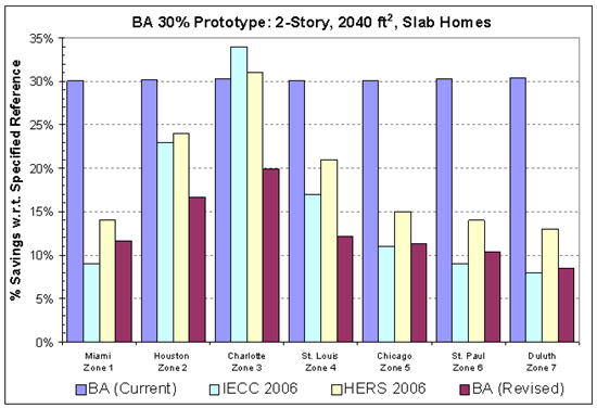
Figure 118. Bar chart showing
the Building America “30% Prototype” home evaluated
using
the
various performance analysis standards that were examined by this study.
Figure 118 provides one example of why it is not possible to state with certainty how the 30% better than Benchmark home compares with either the IECC, HERS ‘99 or even with a hypothetical revised Building America standard [BA (Revised)]. One can calculate the HERS ‘99 Index for these homes from the yellow bars as 1-the % savings. They illustrate that the HERS ‘99 Index for the homes range from 87 in Duluth (not meeting ENERGY STAR standard, which requires a HERS ‘99 Index of 80 or lower in cold climates) to 69 in Charlotte, which is significantly better than ENERGY STAR and, as a matter of fact, which qualifies for the $2,000 tax credit!
While the BA (Current) standards are very consistent at 30% savings across all climate zones, as Figure 1 shows, there simply is no correlation between that BA figure of merit and any of the other figures of merit evaluated by this study.
This study provides additional examples of differences among the standards that are equally disparate. For example, Section 3.3 of the report highlights differences among the standards for number of stories, foundation type, fuel type and home size that illustrate that BA % savings can not be well correlated to the HERS ‘99 Index, even within the same climate.
It is difficult to make recommendations based on this analysis. There can be pros and cons for any given method used to project energy savings. For example, the BA method was originally developed to measure progress toward a set of U.S. DOE energy savings milestones called Joules. The intent was to have a consistent standard of performance tied to mid 1990’s era home standards. However, in the mid 1990’s there were no definitive code standards for windows that are analogous to those that became effective in 1998. In addition, there were no standards or methods in the mid 1990’s for the evaluation of distribution system efficiency, mechanical ventilation or lighting and appliances in homes.
Since the original objective of this study – to establish a correlation between the BA % savings value and the HERS ‘99 Index value – could not be accomplished, there appear to be three potential options for moving forward. While options may not be considered recommendations in the conventional sense of the term, they, along with their advantages and disadvantages, are presented below:
I. Maintain the current BA rule set. This option allows BA program milestones to continue to be measured from a constant reference point. While this reference point can not be directly correlated to current codes or to the HERS ‘99 Index, it does allow program goals to remain consistent with past objectives. However, this advantage also works as a disadvantage. Potential builder partners can not be told with certainty how much better than code their homes will be as the savings with respect to minimum code standards varies greatly with climate. Thus, builder partners are left in a bit of a quandary as to how they can advertise these homes in a way that can be simply explained to their potential customers.
II. Revise the BA rule set. While revising the BA rule set may bring it more in line with alternative, more current rule sets, the analysis presented here did not show that this would result in a complete correlation between the revised BA % savings values and the HERS ‘99 Index (or Code e-Ratio). The revised BA rule set examined here consistently resulted in lower % savings values than the HERS ‘99 rule set. Thus, adopting the revised BA rule set used in this analysis would cause the BA program goals to appear significantly more difficult than code-based programs.
III. Migrate to the HERS ‘99 Index. A large disadvantage of migrating to the HERS ‘99 Index is that it would change the basis of BA program savings goals and milestones. Of course, the previous option, revising the BA rule set, would do the same. There are, however, some advantages of this option. The HERS ‘99 Index is widely used as a performance metric. It is used as the basis for the ENERGY STAR new homes program and other emerging national programs like USGBC’s pilot LEED-H program. The HERS ‘99 rule set also forms the basis for the EPAct 2005 federal tax credit for highly efficient new homes.
As a metric, the HERS ‘99 Index includes all of the energy uses of a home. This is one of the basic tenets of the BA program – that whole home energy use forms the basis of the program. While changing the BA program standard to the IECC rule set would violate this tenet, changing to the HERS ‘99 rule set standard would not. The HERS ‘99 rule set a methodology to “score” the use of on-site energy production, whether by solar, wind or other “free” fuel resources or by highly efficient on-site conventional fuel technologies like micro-turbines and small combined heat and power plants. A significant advantage of the HERS ‘99 rule set standard is that it is a consensus-based national standard.
A disadvantage of the HERS ‘99 Index is that the “scoring method” used by the rule set does not use energy use as the metric. The metric used by the HERS ‘99 rule set is called the normalized modified loads method. It was derived as a compromise consensus method of avoiding the fight between site energy use and source energy use. It can be shown to reasonably reflect energy cost in a market where the ratio between site costs for electricity and natural gas are near the ratio of 3 to 1.
Finally, one advantage of using the HERS ‘99 Index is that it can be explained fairly simply – the “American Standard New Home” has an index of 100 and a home that uses no purchased energy has an index of 0. In other words, zero is zero and anything greater than 100 probably doesn’t meet current minimum energy standards.
Cooling Performance Assessment
of Building America Homes
Paper: Chasar, D., Chandra, S., Parker, D., Sherwin, J.,
Beal, D., Hoak, D., Moyer, N., McIlvaine, J., "Cooling Performance Assessment
of Building America Homes", Fifteenth Symposium on Improving Building
Systems in Hot and Humid Climates, July 24-26, 2006 Orlando, FL.
As of 2004, 46% of new single-family homes are currently built in the South where air conditioning makes up the largest portion of the annual electric bill (USDOE 2005). Through systems engineering, significant reductions in cooling energy have been successfully achieved in these climates by rigorous application of cooling load reduction strategies. Lower cooling loads lead to smaller air conditioners which, when coupled with high efficiency equipment, have led to reductions of over 70% in cooling energy use.
Long-term monitoring of building energy use and environmental conditions has been a strong component of FSEC research since the 1980s. Fully-automated data collection, verification, archiving and management ensure accurate logging of large amounts of data simultaneously from numerous field sites prior to being made available for analysis and display via the internet. Homes are typically monitored using 15 to 50 channels of data to measure indoor and outdoor environmental conditions and energy use of heating, cooling, water heating, whole house, and other points (e.g. Solar PV or Solar DHW) if needed.
Energy performance in many Building America homes has been documented with measured data collected over several years to verify savings projections. An evaluation of measured cooling performance is presented with data from nine homes in three climate regions. Data from potential zero energy homes and minimum code homes provide upper and lower performance bounds.
The nine homes in this comparison study were:
Data Plotting Methodology
Comparisons are based on regression analysis of daily cooling energy per 1,000 square foot of floor area versus average daily temperature difference (outdoor-indoor).
In all of the studied homes, the cooling equipment consisted of split systems with ducted central air handlers. Sub-metered energy from the condenser and air handler was stored at 15 minute intervals and subsequently combined and totaled on a daily basis during the summer months of various years from 1998 to 2005. Daily cooling energy totals were then divided by the total conditioned area of the home to arrive at daily cooling energy per 1,000 square feet. This provided a means of comparing all homes which range from 1,200 to 4,200 square feet.
The daily cooling energy totals were plotted against average daily temperature difference between outdoors and indoors. Weather stations installed at each site collected dry bulb temperature, relative humidity and solar radiation. Indoor temperatures were taken at or very near the thermostat. The x-axis for each data set consists of the difference between the daily average outdoor and indoor temperatures for the 24 hour period starting at midnight. The values generally fell between negative 10 and positive 15 degrees (outdoor minus indoor). Those residences with lower thermostat settings were characterized by large positive values during the hot summer months. The use of temperature difference is intended to account for both indoor and outdoor temperature variations due to occupant determined thermostat settings and outdoor weather variations.
One pair of homes in the data set can be compared without the generalizations discussed above (except for indoor set point) as they were constructed together with identical floor plans and orientation. These two dwellings located in Lakeland, Florida only differed in equipment efficiency and construction. One was built to minimum code requirements while the other was extensively engineered for reduced cooling load and high efficiency. The original measured results from this 1998 project have since formed the basis for the national Zero Energy Homes program (Parker 1998). The pair effectively sets the upper and lower bounds of the data plotted here.
Baseline For Comparison
A single baseline was needed to provide a common comparison point for cooling performance in the eight research houses. This was achieved with data from two minimum-code homes located in Central Florida. The Lakeland home provided the majority of this data collected over five summers from 1998 to 2002. The other home contributing to the baseline was a code-minimum frame structure located in Cocoa, Florida; built in 1991. Data from this home was collected over three summers from 2002 to 2004. Each of these residences is cooled by the originally installed, minimum efficiency equipment, SEER 10 in Lakeland and SEER 9 in Cocoa.
Performance Comparison
The Lakeland high efficiency home was the oldest of those studied (8 years), yet it continues to set the bar for cooling efficiency. The data shown in Figure 119 is typical of the last two years of data collection (2002 & 2003) and represents 72% less cooling energy use than the baseline. While newer the research houses have higher efficiency and sometimes dual-speed cooling equipment, this particular home took advantage of well-designed cooling reduction strategies coupled with a smaller 2-ton cooling system.
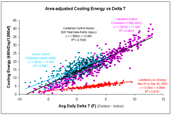
Figure 119. Data and trendlines from two control and one efficient home
Conclusions
Field-collected home performance measurements are needed to gauge progress toward the Building America goal of 70% whole house efficiency. The method developed here made use of measured cooling energy and temperature data analyzed through least-squares linear regression on both code-minimum and research homes. Figure 120 directly compares the linear regression of each data set.
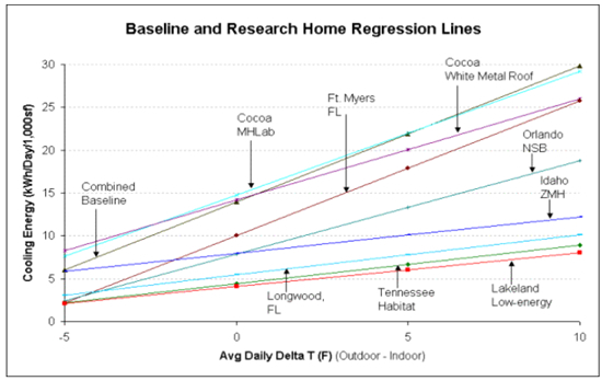
Figure 120. Trendline comparison of Combined Baseline and 8 Research Homes
The cooling energy savings of each research home was determined in reference to a combined baseline established with data from two homes built to minimum code. While the baseline houses do not necessarily represent “typical” code-minimum homes, they nonetheless provide a useful baseline for comparison of the eight research houses. Additional data from homes built to standard construction practices are needed to further refine the baseline.
Additional work is required to determine the influence of home size on cooling performance level. A greater number of people and equipment per square foot tends to concentrate internal loads in smaller homes more so than in larger ones. This may partially explain the MHLab performance, which was below the baseline despite its efficient design. The MHLab was 34% to 62% smaller than the other research homes in the same climate (Florida).
Further research on the influence of ground-coupling on cooling performance will improve the accuracy of comparisons between homes in different climate regions and with different levels of ground contact. All but three homes in this study were of slab-on-grade construction. The basement design of the smallest research home (Tennessee Habitat) was likely a strong contributor to its excellent performance, just as the crawlspace design of the MHLab negatively impacted its cooling efficiency.
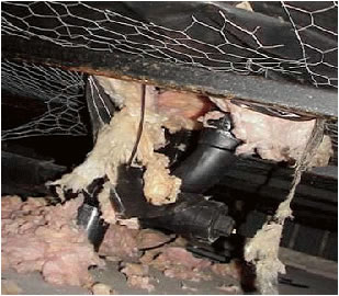
BAIHP Home | Overview | Case Studies | Current Data
Partners | Presentations | Publications | Researchers | Contact Us
Copyright © 2002 Florida Solar Energy Center. All Rights Reserved.
Please address questions and comments regarding this web page to BAIHP Master