


Measured And Predicted Energy Savings
From
An Industrialized House
Armin Rudd
Srinivasa Katakam
Subrato Chandra
Florida Solar Energy Center
Cape Canaveral, FL 32920
ABSTRACT
Side-by-side energy testing and monitoring was conducted on two houses in Louisville, KY. Both houses were identical except that one house was constructed with conventional U.S. 2x4 studs and a truss roof while the other house was constructed with stress-skin insulated-core panels for the walls and second floor ceiling. Air-tightness testing included fan pressurization by blower door, hour-long tracer tests using sulphur hexafluoride, and two-week-long time-averaged tests using perfluorocarbon tracers. Thermal insulation quality testing was done by infrared imaging. Pressure differential testing resulted in recommendations to use sealed combustion appliances, and to increase return air flow from closed rooms. By calculation, the conductive building load coefficient (UA) differed by only 2% between the two houses. Heating energy-use monitoring showed savings for the panel house of 12% with electric heating and 15% with gas heating. A comparison of the two monitoring periods showed that the combined efficiency of the gas furnace and air distribution system for both houses was close to 80%. Measured energy-use regression models with Typical Meteorological Year weather data gave a prediction of seasonal energy savings of 16% for electric heating and 19% for gas heating. Seasonal heating energy-use predictions were also made with the DOE2.1E hourly building energy simulation program which gave savings of 7% for electric heating and 6% for gas heating. The discrepancy between savings predicted by measurement and simulation may be related to rated performance versus field performance of insulation systems. From the data, it appears that this type of industrialized construction has energy efficiency advantages over conventional construction.
INTRODUCTION
Background
Stressed-skin insulated-core (SSIC) panels are gaining favor in the residential construction industry as an alternative to conventional stud-frame construction. SSIC panels most generally consist of two layers of oriented strand board (OSB) as structural skins separated by foam insulation. The panels are manufactured, and sometimes machined for openings and angle cuts, in a factory, increasing the potential for cost savings through industrialization. Various splining and connection methods are used on-site to assemble the panels into a building envelope. A distinct energy advantage of the panel construction is that the insulation is less interrupted by framing and air movement within the insulation is not possible.
Scope
A side-by-side evaluation was conducted to assess the heating energy-use benefits of using SSIC panels in residential construction in Louisville, Kentucky, U.S.A. (Rudd 1994) (Note: This paper includes additional information resulting primarily from analysis of hourly simulations). One house was constructed as a conventional U.S. 2x4 stud-frame, and the other was constructed with SSIC panels. The SSIC wall panels were 4 feet wide by 8 feet high and 2x4 lumber was used for the vertical spline. The SSIC ceiling panels were 4 feet wide by 16 feet long and 2x8 lumber was used for the spline. Since the solid lumber splines extended between the interior OSB skin to the exterior OSB skin, they created more of a thermal short than other splining methods used with the SSIC technology. Both houses were privately financed and constructed by the same builder who has experience with both types of construction. The builder was not coached to build either house differently, better or worse, than he normally would. Each two-story house has 1200 ft2 floor area and has the same floor plan, elevations, orientation, and nearly the same exterior colors. Both houses are heated by natural gas furnace. All the air distribution ducts are within the thermal envelope of the building. A comparison of the basic building parameters for the two houses is given in Table 1. Energy testing and unoccupied monitoring with simulated occupancy was conducted. Hourly simulations were run to compare to measured energy-use data and to make seasonal energy-use predictions.
Table 1. Thermal envelope parameters of the stud-frame
(SF) and
stressed-skin insulated-core (SSIC) panel houses
| Component | House Type | Construction Type | Insulation |
| Foundation | Both | Block stem wall and slab | R-10 to 2 foot depth |
| Walls | SF SSIC |
2 x 4 stud 3-5/8" EPS core panel |
R-13 fiberglass batt Partial R-3.5 sheathing R-14 EPS core |
| Windows | Both | Double glazed, wood frame, aluminum cladding |
R-2.0 |
| Second floor ceilings |
SF
SSIC |
2 x 4 truss
Flat, 7-3/8" EPS core |
R-30 loose-fill cellulose
R-29 EPS core |
METHODOLOGY
Both houses were designed to have a conductive thermal transmittance (UA) equal to each other. Calculations, using the as-built configuration and thermal transmission data from a reference handbook (ASHRAE 1989), showed that the SSIC panel house conductive UA was 265 Btu/hr-oF and the frame house conductive UA was 271 Btu/hr-oF, a difference of only 2%. Figures 1a and 1b show the conduction heating load distribution for the stud-frame house and the SSIC panel house, respectively. When the measured infiltration UA was included, from the average of all air tightness testing results shown in Figure 2, the total building UA for the panel house was 5% lower than that of the frame house. Air infiltration made up 15% and 12% of the total heating load for the frame and panel houses, respectively.
Five days of building diagnostics testing was performed on each house. The testing assessed thermal insulation quality by infrared imaging, building envelope and air distribution system air-tightness by fan pressurization and tracer gas, pressure effects inside the house due to interactions of the air distribution system, calculated versus measured building load coefficients by co-heating, and building thermal decay by cool-down.
Four weeks of short-term energy-use monitoring was conducted, including two weeks of electric heating energy-use monitoring and two weeks of gas heating energy-use monitoring. The houses were unoccupied during monitoring. In addition to measurement of heating energy-use, measurements of house dry bulb temperature, mean radiant temperature, south wall surface temperature, and relative humidity were continuously monitored. Passive perfluorocarbon tracer gas sources and samplers were deployed to measure the time-averaged house air exchange rates (Dietz 1986). A weather measurement station was installed on top of the SSIC house and continuously monitored dry-bulb temperature, relative humidity, global horizontal and global south-facing vertical solar radiation, wind speed and wind direction.
Two regression models were employed to fit the daily heating energy-use data. The first model included only two coefficients:
y = a1*(Tin - Tout) +a2
where: y = heating energy-use
Tin = inside temperature
Tout = outside temperature
a1, a2 = regression coefficients
The second model included a third coefficient to pick up the impact of solar gain:
y = aO* Ihor + a1 * (Tin - Tout)
+ a2
where: Ihor = horizontal solar irradiance
The regression models were used to make a prediction of seasonal energy-use by applying TMY weather data to the models.
In addition, the DOE2.1E hourly building energy simulation program was employed to predict seasonal heating energy-use. The initial intent was to "calibrate" the simulation model by inputing measured on-site weather data and comparing the simulation energy-use output to the measured energy-use. If agreement was poor, the model would be evaluated to find the possible causes and make adjustments as reasonable (Lutz 1992). Editing the solar radiation part of the weather file for input to the simulation proved to be problematic and was not accomplished. More work is on-going in this area. Heating energy-use predictions by the DOE2 simulation are given here for three cases: (1) Seasonal (November thru March) heating energy-use with original TMY weather file, and the average measured air change rate for both houses; (2) Seasonal heating energy-use with original TMY weather file, and 0.35 ACH air change rate for both houses; and (3) Partial season (actual monitoring periods) energy-use using a TMY weather file with fields edited for measured air temperature, dewpoint, wind speed and wind direction, with the average measured air change rate for both houses.
RESULTS
Energy Testing/Building Diagnostics
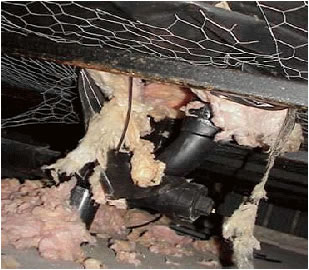
Infrared scanning indicated that the thermal insulation quality of both houses was good. Few defects were found which would have a significant impact on energy use. The stud-frame house had two insulation defects that are worth noting. One defect involved a ceiling area over the stairwell, approximately 6 ft2, where the blown-in insulation was missing. The other defect became apparent only after infiltration was forced by the blower door--an air leak occurred where the exhaust duct in the first floor bathroom penetrated the band joist and was not completely sealed. Examination of a photograph of that same penetration, taken during construction, revealed that a worker had attempted to seal the gap, but he did not get it sealed well enough. These defects were not fixed.
Air-tightness was evaluated for the building envelopes and the air distribution systems. Blower door and tracer gas tests showed that, on average, the envelope of the SSIC panel house was 22% more air-tight. The tracer gas tests, using SF6 and a specific vapor analyzer, showed that both houses had an increase in air infiltration when the air distribution system was operating. However, duct leakage to the outdoors was less than the blower door could measure accurately. Figure 2 gives a summary of these results. Also included in Figure 2 are results from the perfluorocarbon tracer (PFT) time-averaged infiltration measurements taken during the electric and gas heating monitoring periods. The averaging period was 17 days for electric heating and 21 days for gas heating. PFT results showed higher infiltration for the frame house compared to the panel house and higher infiltration for the gas heating monitoring period compared to the electric heating monitoring period. During the gas heating period, the influence of the natural draft furnace, and the movement of air by the air distribution system, may have contributed to higher infiltration. Also, the average outdoor temperature during the gas heating period was about 6.5oF lower which may have driven more stack-effect infiltration. The wind speed was similar for both periods. Because of the variation in natural air infiltration, as measured by the three methods, the results are somewhat inconclusive in an absolute sense, however, they are consistent in a relative sense in that the panel house was always tighter and air infiltration was always greater when the furnace fan was operating. Both houses were considered to be more air-tight than average houses in the Louisville area, an average of all the air-tightness test results yielded a natural infiltration rate of 0.27 for the frame house and 0.21 for the SSIC panel house. The American Society of Heating Refrigerating and Air-Conditioning Engineers (ASHRAE) Standard 62-1989 recommends that houses should have at least 0.35 air changes per hour or 15 ft3/min of ventilation air per occupant. Based on that, a whole-house fresh air ventilation system should be considered for both the frame and panel houses. For the Louisville climate, an exhaust-only ventilation system providing at least 0.35 air changes per hour, or about 60 ft3/min for these particular houses, may be the most cost-effective. This may be accomplished by installing a two speed exhaust fan in the attic which is ducted to each bathroom and to the outdoors. The fan could run on low speed constantly, and be manually switched to high speed by occupants. A humidistat control could also be linked to the high speed mode. A 100 ft3/min, 48 W fan would use about 420 kW-hr per year to operate continuously. At $0.08/kW-hr the cost would be $34/yr. DOE2.1E simulation results, listed in Table 4, show that raising the air change rate to 0.35 ACH would increase heating energy-use by 345 kW-hr for the frame house and 599 kW-hr for the panel house. Some have questioned why it is recommended to seal a house tightly and then install a fan to ventilate it. The answer is that relying on random leaks in the building, and unknown pressure forces due to wind and temperature, does not assure adequate ventilation at all times, and it may lead to over-ventilation and higher energy bills. In addition, leaky building envelope and air distribution systems can cause pressure imbalances which may lead to moisture accumulation problems or even the malfunction of combustion appliances.
A series of measurements were taken to evaluate pressure differentials within the building, and between the building interior and the outdoors. The impact of building pressure differentials can affect occupant health and safety, building durability, and energy-use. Since both houses have gas furnaces inside the conditioned space, occupant health and safety could be affected if negative pressures caused the furnace to back-draft. Differential pressure measurements taken between the utility closet and the outdoors showed pressures between -2.0 Pa and -5.7 Pa. These measurements were taken with the furnace fan on, and the kitchen and bath exhaust fans on. A clothes dryer, which will be installed inside the house, would have increased the exhaust flow. Since the utility closet has two 6" ducts connecting it to the ventilated attic to provide combustion air and dilution air, the utility closet doors should be weather stripped to better seal the furnace and gas hot water heater from the main body of the house, or use sealed combustion appliances. Additional pressure differential measurements taken between closed rooms and the main body of the house, with the furnace fan and exhaust fans on, showed that the main body depressurized to about -5 Pa while the closed rooms pressurized to between 3 and 10 Pa. These pressure differentials would cause increased infiltration in the main body and increased exfiltration in the closed rooms, resulting in increased energy-use (Cummings 1992). In a cold climate, if warm moist air is forced through the building shell due to pressurized rooms, moisture may condense inside the building shell and cause material degradation. Adequate return air flow from closed rooms could be provided by separate return ducts, or transfer ducts which simply connect closed rooms to the main body with a short duct.
A co-heating test was performed to determine the as-built total UA (building load coefficient, including infiltration). This test monitored the inside-to-outside temperature difference and the electric heating energy used to hold the inside temperature steady. The measured UA for the SSIC panel house was 19% lower than that of the stud-frame house, for the one-night co-heating test. A more accurate estimate of the as-built building UA is presented with the electric heating monitoring results. That UA is calculated by a linear regression of, in effect, 17 nights of co-heating data.
An evaluation of the temperature decay characteristic of each house was made, starting after sundown, by letting the house temperature fall with no internal heat source. The two buildings appear to have similar thermal capacitance. The time constant for the drop in inside temperature as a function of time for the stud-frame house was 8 hours compared to 10 hours for the SSIC panel house. The panel house cooled more slowly due to its lower conductive heat loss rate and lower infiltration rate. In a follow-on test, where the houses were heated up at the same energy input rate, the panel house heated up more quickly.
Energy-use Monitoring
Two periods of energy-use monitoring, one for electric heating and one for gas heating, were included in the monitoring plan in order provide a better comparison of the thermal envelopes of the two houses, and to calculate a total heating system and air distribution system efficiency. Electric heating eliminated the additional measurement uncertainties associated with the gas furnace and the increased air infiltration effects and leakage due to the air distribution system. Since electric heating efficiency is 100%, the difference in measured building UA between the electric heating and gas heating monitoring should be due mainly to the gas furnace efficiency and infiltration/leakage effects caused by the air distribution system.
A total of seventeen consecutive days of electric heating energy-use monitoring was completed. The houses were heated with six 1300 W electric heaters placed throughout the house. The heaters were turned on and off by computer control based on temperature feedback from thermocouples. Data was collected every six seconds and averaged or totalized and stored every 6 minutes. Temperatures typically did not vary more than 0.5oF within the house and between houses. Outdoor temperature for the entire electric heating period averaged 39oF.
A total of 21 days of gas heating energy-use monitoring was conducted. For a seven-day period, there was a gap in gas meter data for the stud-frame house due to a meter failure. Hence, only 14 days of gas heating monitoring were analyzed. The electronic-ignition, gas furnaces were turned on and the thermostats were adjusted to minimize the control dead-band and to keep each house as close as possible to 72o F. The temperature within each house, and between houses, typically did not vary more than 1.5oF. Outdoor temperature during the entire gas heating period averaged 33oF.
Differences in air temperature, south wall temperature, and mean radiant temperature were small for both monitoring periods, indicating that thermal comfort conditions would be similar in both houses. Relative humidity averaged about 2% higher in the panel house, which was within the sensor accuracy limit of ±2%.
A linear regression of the monitored heating energy-use versus inside-to-outside temperature difference was calculated to obtain a more accurate estimate of the as-built building UA than the one-night co-heating test could give. Only night hours 2-7 were included in the regression to minimize the effects of solar gains and thermal capacitance. Residual analysis showed acceptable normality of distribution and no significant bias error. Table 2 gives a summary of the results for both monitoring periods and the one-night co-heating test. The building UA of 276 Btu/hr-oF for the frame house and 242 for the panel house were expected to be the most accurate and repeatable results. Those UA values, compared to those obtained from the gas heating monitoring period, yielded a combined efficiency for the gas furnace plus the air distribution system leakage and possible infiltration effects due to pressure imbalances. Those efficiencies were 78% and 81% for the frame and panel houses, respectively. Since the gas furnaces have a rated 80% Annual Fuel Utilization Efficiency, it seemed that the conclusion from blower door testing, that there was no measurable duct leakage, was confirmed. All interior doors were open during the monitoring periods, hence there was little opportunity for pressure imbalance which could increase building air leakage.
Table 2. Measured Building UA and heating system efficiency
|
Measured Building UA |
|||
|
Frame House |
Panel House |
||
|
(Btu/hr- oF) |
(Btu/hr- oF) |
Percent Difference |
|
| Electric heating monitoring (17 nights) |
276 |
242 |
12.3% |
| Gas heating monitoring (14 nights) |
352 |
300 |
14.8% |
|
Gas furnace and air distribution |
|||
|
78.4% |
80.7 |
||
Heating energy savings were calculated for both monitoring periods by comparing the total energy consumed by each house, less the internal gain profile. No outside lights were operable, and the gas hot water heaters were turned off, hence, all electricity and gas consumed were considered to contribute to the heating of the houses. Table 3 summarizes the heating energy savings results. The night data, hours 2-7, were expected to give the most accurate comparison of the two building thermal envelopes due to the fact that any solar gain differences between the two buildings would have no impact. Night data showed that the SSIC panel house used 12% less heating energy than the stud-frame house with electric heat, and 15% less with gas heat. The daily data was considered to give the next level of accuracy and was primarily utilized to obtain a simple mathematical model with which to predict seasonal savings. Daily data (all 24 hours) indicated that the panel house used 15% less energy with electric heat and 17% less with gas heat. Using the two regression models from Eqs. (1) and (2), seasonal heating energy savings were predicted. The difference in energy savings predicted by both models, using the actual monitored weather data, was less than 0.2%. This regression model analysis showed that solar irradiance had almost no impact on heating energy savings during the monitoring periods. When the regression models were used to extrapolate, or predict seasonal energy savings, using Typical Meteorological Year weather data for Louisville, the difference between the models became more significant. The predicted seasonal heating energy savings was 16% with electric heat and 19% with gas heat, in favor of the panel house.
Table 3. Heating energy savings of SSIC panel house over stud-frame house
|
Percent heating |
|
| Electric Heating Monitoring Night data Daily data Seasonal predicted (regression model) Gas Heating Monitoring |
|
Table 4 lists average daily energy use, maximum daily energy use, total energy use, and percent difference in total energy use for the electric heating monitoring period, and the various analysis methods described. In addition to the measured data regression model results, energy-use predictions from the DOE2.1E hourly building energy simulation program are also listed. One should note that since the total heating load for both houses is not large, the absolute energy savings is modest even though the percent savings is significant. The bar chart in Figure 3 illustrates the seasonal heating energy-use difference in kilowatt-hours for the measured data regression model and the DOE2.1E simulation. Two sets of air change rates were simulated: (1) the average of the measured rates (shown in Figure 2), and (2) the ASHRAE Standard 62-1989 rate of 0.35 air changes per hour. In the first case, the simulation predicted 7% seasonal savings for the panel house with electric heat, and 6% savings with gas heat. When the higher air change rate was used, assuming mechanical ventilation for both houses, the simulation predicted only 2% energy savings for the panel house.
Using actual measured weather data as input (except solar radiation), the simulation model under-predicted (compared to measured results) heating energy use during the two monitoring periods. It under-predicted by 20% for the frame house and 11% for the panel house, for the electric monitoring period. For the gas heating monitoring period, the simulation model under-predicted by 20% for the frame house and 7% for the panel house. The fact that the simulation under-predicted actual energy use significantly more for the frame house than for the panel house may raise questions about the field performance of "loose" insulation systems versus their rated performance (Custom Builder 1994). This issue should be studied more fully, perhaps with calibrated hot bot tests with an imposed air pressure differential and a vapor pressure differential across the test wall.
CONCLUSIONS
Extensive energy-use testing and monitoring was conducted comparing the building thermal envelopes of a conventional stud-frame house and an industrialized house using stressed-skin insulated core panels for its walls and ceiling. The houses were otherwise identical. By calculation, the two houses had a conductive thermal transmittance within 2% of each other. Monitored heating energy-use data, for night hours 2-7, showed that the SSIC panel house used 12% less energy than the frame house with electric heating, and 15% less with gas heating. Full-day (all hours) data gave 15% electric heating savings and 17% gas heating savings for the panel house. Prediction of seasonal heating energy savings, using a regression model and TMY weather data, indicated savings of 16% with electric heat and 19% with gas heat. A hourly building energy simulation model (DOE2.1E) predicted seasonal heating energy savings of 7% and 6% for electric and gas heat, respectively. In addition to the panel house being more air-tight, there seem to be other factors, possibly such as field performance versus rated performance of insulation systems, which cause the panel house to use less heating energy. These factors require further investigation. From the data, it appears that this type of industrialized construction has energy efficiency advantages over conventional construction.
ACKNOWLEDGEMENTS
This research was conducted as part of the Energy Efficient Industrialized Housing Project funded by the U.S. Department of Energy, George James, program manager. The authors thank the Structural Insulated Panel Association, and specifically Frank Baker and Fred Fischer, for their efforts in support of this research. The authors also acknowledge the valuable contributions made by Philip Read of FSEC and Michael Johnston of Dovetail Construction, the builder of both houses.
REFERENCES
ASHRAE. 1989. Handbook of Fundamentals. American Society of Heating, Refrigeration and Air-conditioning Engineers, Atlanta, GA.
Cummings, James B., John Tooley, Neil Moyer. 1992. "Duct Doctoring: Diagnosis and Repair of Duct System Leaks." Under contract to Florida Energy Office. Florida Solar Energy Center, Cape Canaveral, FL.
Custom Builder. 1994. "Housewraps Are Put To The Test." Jan/Feb, pp. 9.
Dietz, Russell N., Robert W. Goodrich, Edgar A. Cote, Robert F. Wieser, 1986. "Detailed Description and Performance of a Passive Perfluorocarbon Tracer System for Building Ventilation and Air Exchange Measurements." Measured Air Leakage of Buildings. ASTM STP 904, H.R. Trechsel and P.L. Lagus, Eds., American Society for Testing and Materials, Philadelphia, pp. 203-264.
Lutz, Jim, 1992. "Simulation Software Gets Reality Check." Home Energy, Sep/Oct, pp.21.
Rudd, Armin, and Subrato Chandra. 1994. "Side-By-Side Evaluation Of A Stressed-Skin Insulated-Core Panel House And A Conventional Stud-Frame House," Proceedings from the 1994 EEBA Excellence Conference, pp. A-106 - A-122, Energy Efficient Building Association, Wausau, WI.
BAIHP Home | Overview | Case Studies | Current Data
Partners | Presentations | Publications | Researchers | Contact Us
Copyright © 2002 Florida Solar Energy Center. All Rights Reserved.
Please address questions and comments regarding this web page to BAIHP Master