|
BAIHP
Research:
C. Field and Laboratory Building Science Research
Cont'd
To determine the impact of air handler location on heating
and cooling energy use, researchers measured the amount of
air leakage in air handler cabinets, and between the air
handler cabinet and the return and supply plenums. To assess
this leakage, testing was performed on 69 air conditioning
systems. Thirty systems were tested in the 2001 and 39 in
2002. The 69 systems were tested in 63 Florida houses (in
six cases, two air handlers were tested in a single house)
located in seven counties across the state - four in Leon
County in or near Tallahassee, 17 in Polk County, three in
Lake County, 13 in Orange County, one in Osceola County,
two in Sumter County, and 29 in Brevard County. All except
those in Leon County are located in central Florida. Construction
on all houses was completed after January 1, 2001, and most
homes were tested within four months of occupancy.
In each case, air leakage (Q 25) at the air handler and
two adjacent connections was measured. Q 25 is the amount
of air leakage which occurs when the ductwork or air handler
is placed under 25 Pa of pressure with respect to its surrounding
environment. Q 25 also can be considered a measurement of
ductwork perforation.
To obtain actual air leakage while the system operated,
it was necessary to measure the operating pressure differential
between the inside and outside of the air handler and adjacent
connections. In other words, it was necessary to know the
perforation or hole size and the pressure differential operating
across that hole. By determining both Q 25 and operating
pressure differentials, actual air leakage into or out of
the system was calculated.
Field Testing Leakage Parameters
Testing was performed on 69 air conditioning systems to
determine the extent of air leakage from air handlers and
adjacent connections. Testing and inspection was performed
to obtain:
- Q 25 in the air handler, Q 25 at the connection to the
return plenum, and Q 25 at the connection to the supply
plenum.
- Operating pressure at four locations - the return plenum
connection, in the air handler before the coil, in the
air handler after the coil, and at the supply plenum connection.
- Return and supply air flows were measured with a flow
hood. Air handler flow rates were measured with an air
handler flow plate device (per ASHRAE Standard 152P methodology).
- Overall duct system and house airtightness in 20 of
the 69 homes.
- Cooling and heating system capacity based on air handler
and outdoor unit model numbers.
- The location and type of filter.
- Dimensions and surface area of the air handler cabinet.
- The fractions of the air handler under negative pressure
and under positive pressure.
- The types of sealants used at air handler connections.
- Estimated
portion of the air handler leak area that was sealed “as
found.”
Air
Handler Leakage
|
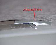
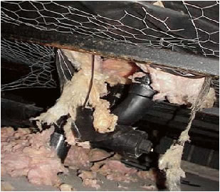
Figure
78 Thermograph
of air being drawn
from the attic to the air handler
in a Florida house |
Leakage in the air handler cabinet averaged 20.4 Q 25 in
69 air conditioning systems. Leakage at the return and supply
plenum connections averaged 3.9 and 1.6 Q 25, respectively.
Using the operating pressures in the air handler and at the
plenum connections, these Q 25 results convert to actual
air leakage of 58.8 CFM on the return side (negative pressure
side) and 9.3 CFM on the supply side (positive pressure side).
The combined return and supply air leakage in the air handler
and adjacent connections represents 5.3% of the system air
flow (4.6% on the return side and 0.7% on the supply side).
This is a concern, when considering that a 4.6% return leak
from a hot attic (peak conditions; 120 oF and 30% RH) can
produce a 16% reduction in cooling output and 20% increase
in cooling energy use (Cummings and Tooley, 1989), and this
was only from the air handler and adjacent connections. (Figure
78)
“Total” Duct
Leakage
Some important observations were made from the extended
test data in 20 houses. Total leakage on the return side
of the system (including the air handler and return connection)
was 53 cfm with weighted operating pressure on the return
side of about -100 Pa (including the air handler), operating
return leakage was calculated to be 122 CFM, or 9.7% of the
rated system air flow.
Total
leakage on the supply side of the system (Q 25s,total)
was very large, at 134. The ASHRAE 152P method suggests
using half of the supply plenum pressure as an estimate
of the overall supply ductwork operating pressure, if the
actual duct pressures are not known. For the 20 systems
with extended testing, supply plenum pressure was 73.3
Pa. Based on a pressure of 37 Pa, actual leakage should
be 167 CFM or about 13.3% of the rated air flow. To test
the ASHRAE divide-by-two method, supply duct operating
pressure measurements were taken from 14 representative
systems. These averaged 35.9 Pa, compared to 65.7 Pa for
the supply plenums for those same 14 systems. For these
systems, the duct pressure was 55% of the supply plenum
pressure - making the ASHRAE method a reasonable method
for estimating central Florida home’s supply ductwork
operating pressures.
However,
the ASHRAE method wasn’t reasonable for
estimating central Florida home’s return ductwork operating
pressures. For these 20 systems, 38% of the Q 25r,total was
in the air handler and 62% of the Q 25r,total was in the
return ductwork. Given an air handler pressure of -133 Pa,
a return plenum pressure of -81.5 Pa, and return duct pressure
of approximately -70 Pa, the weighted return side pressure
was approximately -95 Pa. By contrast, the ASHRAE method
predicted -41 Pa. Clearly, in systems with a single, short
return duct plenum like those commonly found in Florida,
the actual operating pressure should be greater than the
return plenum, maybe by as much as 1.2 times the plenum pressure.
Return side leakage is available on 58 of the 69 systems.
Return leak air flow (Q r,total) combined for the air handler,
return connection, and the return ductwork was found to be
152.4 CFM, or 11.8% of total rated system air flow for this
group. For this larger sample, Q r,total is considerably
greater than for the 20 houses with extended testing. These
alarming results show that even in these newly constructed
homes about 12% of return air and 13% of supply air duct
systems are leaking.
Duct
Leakage to “Out”:
In
20 homes, duct leakage to “out” was measured. (Table
45) On average, 56% of the leakage of the return ductwork
and supply ductwork was to “out.” “Out” is
defined as outside the conditioned space, including buffer
spaces like an attic or garage. The fraction of leakage
that was to “out” varied by air handler location.
For return ductwork, the proportion of total leakage to “out” is
81.4% for attic systems, 67.6% for garage, and 28.0% for
indoors. For supply ductwork, the proportion of total leakage
to “out” was in the range of 52% to 56% for
all three locations.
Table
45 Portion of duct leakage to outdoors [(Q 25,out/Q
25,total) * 100] |
Air Handler Location |
Return |
Supply |
Entire Duct System |
Attic |
81.4% |
56.5% |
63.2% |
Garage |
67.6% |
51.7% |
56.0% |
Indoors |
28.0% |
52.6% |
37.1% |
The
attic return ductwork was the most predictive variable
to “out” leakage findings. All of the return
ductwork for attic units was located in the attic. Much of
the return ductwork for other units was located in the house.
As a consequence, the energy penalty associated with locating
the air handler in the attic was greater than indicated in
the computer modeling results in Table 46, since
the modeling only considered the leakage of the air handler
cabinet and the adjacent connections, and not the return
ductwork leakage.
Table
46 Duct leakage “total” and
to “out” for three locations, for
both 25 Pa test pressure and for actual system
operating pressure. Sample size is in [brackets] |
| . |
Attic
(cfm) |
Garage
(cfm) |
Indoors
(cfm) |
Combined
(cfm) |
Test |
Total |
Out |
Total |
Out |
Total |
Out |
Total |
Out |
Q 25,r [58] |
61.9 |
50.4 |
93.3 |
63.1 |
67.8 |
19.0 |
75.7 |
44.9 |
Q 25,s [20] |
109.1 |
61.6 |
170.6 |
88.2 |
119.5 |
62.9 |
134.3 |
71.4 |
Q r [58] |
118.1 |
96.1 |
194.4 |
131.4 |
134.6 |
37.7 |
152.4 |
90.4 |
Q s [20] |
135.6 |
76.6 |
212.0 |
109.6 |
148.5 |
78.1 |
166.9 |
88.7 |
Table 46 shows
that the operating supply leakage to “out” was large for all three air handler
locations, averaging 89 CFM. The average operating return
leakage to “out” was slightly larger, at 90 CFM.
However, there was a large variation between air handler
locations; 96 CFM for attic systems, 131 CFM for garage systems,
but only 38 CFM for indoor systems. From an energy perspective,
the attic systems experienced the greatest “real” energy
penalties, because all of the return ductwork and air handlers
were located in the attic. (Table 45) By contrast,
a majority of the return leakage for the garage systems likely
came from the garage (which is considerably cooler than the
attic). For indoor systems, the return leakage to “out” most
likely originated from the attic. However, since the return
leakage was so much smaller, the energy impact was likely
considerably less than both the attic and the garage systems.
|
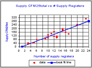
Figure
79 Supply CFM25 “total” leakage
versus the number of supply registers. |
|
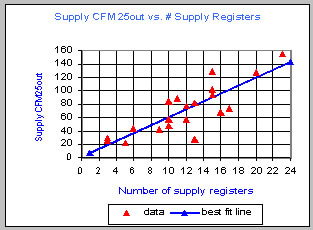
Figure
80 Supply CFM25 “out” leakage
versus the number of supply registers. |
Correlation
of Supply Duct Leaks with Number of Registers: When
analyzing the supply leakage in the extended test data,
a surprising correlation was observed. This correlation
indicated a systematic and consistent duct fabrication
problem across a wide range of air conditioning contractors. Figure
79 illustrates this correlation, showing that each
supply duct has a remarkably predictable total duct leakage.
The coefficient of determination is 0.86, indicating that
86% of the variability in total supply duct leakage was
explainable by the number of supply registers. Figure
80 shows a similar relationship between supply leakage
to “out” and the number of supply registers.
In this case the coefficient of determination was 0.69,
indicating that 69% of the variability in total supply
duct leakage was explainable by the number of supply registers.
Note that one of the two houses with 13 registers showed
considerably less leakage than expected. In this case, supply
ducts were located in the interstitial space between floors.
When the house was taken to -25 Pa, it is probable (though
not measured) that the interstitial spaces were substantially
depressurized as well, so leaks in those supply ducts would
show less air flow (i.e., less pressure differential = less
leakage air flow) and therefore be under-represented.
|
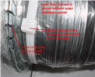
Figure
81 Flexible duct to metal
collar connection. |
|
|
Figure
82 Gaps at the
supply register to drywall joint |
The data suggest that a duct leakage problem occurs in
nearly all new homes. Researchers identified three issues
that create most of the leakage: (1) the connection of the
supply register or return grill (Figure 82), (2)
the boot (supply box) to sheet rock connection (Figure
81), and (3) the flex duct to collar connection. The
supply register or return grill leakage typically shows as
supply leakage in the “total” test. It usually
occurs when the register or grill does not fit snugly to
the ceiling or wallboard. Issues two and three show up as
leakage to both “out” and “total.”
Figure
81 shows how flexible duct connections typically are
made. In some cases metal tape is used, but the tape wrinkles
when applied to complex angles and over bumps associated
with these connection types. Although small in size, these
cumulative wrinkles at each connection allow air to pass
through.
Computer
Modeling for Florida Energy Code Air Handler Multipliers:
FSEC
researchers performed simulations and developed air handler
multipliers for the Florida Energy Code using this study’s
simulation results. Researcher used the FSEC 3.0 model,
a general building simulation program developed in 1992.
This program provided simultaneous detailed simulations
of a whole building system, including energy, moisture, multi-zone
air flows, and air distribution systems.
In 2001, modeling had been performed to develop initial
air handler multipliers. These multipliers were based on
estimated Q 25 and duct operating pressures. At the time
of the 2001 modeling, there was essentially no data on air
handler and connection leakage. Modeling for this project
was performed again, but this time using the results of the
69 field tested homes.
The modeling inputs used in 2001 and those from the current
study are shown below. (Table 47) Note that the
same Q 25 and operating depressurization (dP) values was
used for all air handler locations, since there was essentially
no difference between the Q 25 values for attic, garage,
and indoor air handler locations when gas furnace units were
removed from the analysis.
Table
47 Air Handler (AH) And Connection Inputs For 2001
And
Current Project Computer
Modeling
|
| . |
2001 Q 25 |
AH Study Q 25 |
2001 dP |
AH Study dP |
Return connection |
8.7 |
3.9 |
-40 |
-86.1 |
AH – depressurized
portion |
48.5 |
17.6 |
-42 |
-139.1 |
AH – pressurized
portion |
9.6 |
2.8 |
43 |
106.5 |
Supply connection |
7.8 |
1.6 |
32 |
58.2 |
Total |
74.6 |
25.9 |
. |
. |
While the Q 25 leakage for the air handler and connections
was about 65% less than earlier estimates, operating pressures
were much higher. The air handler multipliers based on the
current computer modeling results are presented in Tables
48, 49, and 50. Modeling of air handler energy use also
was performed for the air handlers located outdoors, despite
the fact that no field data was collected for outdoor units.
The modeling input parameters were the same as the other
air handler locations as shown in Table 47. Note
also that the air handler multipliers for the attic, indoors,
and outdoors are normalized to the garage, since this location
was considered the baseline. The final report for this study
can be viewed online at: http://www.fsec.ucf.edu/bldg/pubs/cr1357/index.htm.
Table
48 Florida Energy Code AH Multipliers for South Florida |
AH Location
|
Winter |
Summer |
Old |
2001 |
new |
old |
2001 |
new |
attic |
1.04 |
1.15 |
1.12 |
1.04 |
1.09 |
1.06 |
garage |
1.00 |
1.00 |
1.00 |
1.00 |
1.00 |
1.00 |
indoors |
0.93 |
0.91 |
0.94 |
0.93 |
0.91 |
0.92 |
outdoors |
1.03 |
1.08 |
1.06 |
1.03 |
1.03 |
1.01 |
Table
49 Florida Energy Code AH Multipliers for Central
Florida |
AH Location
|
Winter |
Summer |
Old |
2001 |
new |
old |
2001 |
new |
attic |
1.04 |
1.11 |
1.08 |
1.04 |
1.10 |
1.08 |
garage |
1.00 |
1.00 |
1.00 |
1.00 |
1.00 |
1.00 |
indoors |
0.93 |
0.92 |
0.94 |
0.93 |
0.90 |
0.92 |
outdoors |
1.03 |
1.09 |
1.05 |
1.03 |
1.02 |
1.01 |
Table
50 Florida Energy Code AH Multipliers for North Florida |
AH Location
|
Winter |
Summer |
Old |
2001 |
new |
old |
2001 |
new |
attic |
1.04 |
1.10 |
1.03 |
1.04 |
1.11 |
1.08 |
garage |
1.00 |
1.00 |
1.00 |
1.00 |
1.00 |
1.00 |
indoors |
0.93 |
0.93 |
0.94 |
0.93 |
0.91 |
0.92 |
outdoors |
1.03 |
1.07 |
1.02 |
1.03 |
1.02 |
1.01 |
Purpose
|
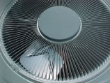
Figure
83 Air conditioning
condenser fan and diffuser. |
The purpose of this study is to develop an air conditioner
condenser fan that reduces the electric energy use of
the condensing unit (Figure 83). To accomplish
this, researchers are designing and producing more aerodynamic
fan blades and substituting smaller horsepower (HP) motors
which achieve the same air flow rates as the larger,
less efficient motors typically used.
4
th Budget Period
During
the 4th budget period, researchers developed baseline data
for the fan power use in a standard condensing unit (Trane
2TTR2036) and tested a new prototype design: “Design
A5” with five asymmetrical blades
Baseline
data included condenser airflow, motor power, sound levels,
and condenser cabinet pressures. Test results favorably
compared with the manufacturer’s test
data. An experimental set of fan blades, “Design-A5,” designed
for a 1/8 hp motor at 850 rpm was numerically created
and then successfully produced using rapid prototyping.
These prototype blades were substituted on the original
condenser, and all test measurements were redone. Design-A5
was found to reduce power use by 20% (40 watts) with
approximately equivalent airflow to the original condensing
blade design.
5 th Budget Period
During the 5th budget period, activities included re-calibration
and improvement of the test equipment configuration,
refinement of various designs, and patent filing.
Re-calibration and Improvement of Test Equipment
Configuration
The
air flow measurement equipment was re-calibrated by the
Energy Conservatory in Minneapolis in accordance with ANSI/ASHRAE
51-1985 ("Laboratory Methods of
Testing Fans for Rating."). Testing determined that
the "flow cube" could be modified with settling
screens and a flow straightener to yield a 5% absolute
flow accuracy and a 2% relative accuracy from the test
equipment. Also, the test configuration was moved indoors
in order to better measure sound and also to reduce
test variability from wind-related effects. Noise measurement
protocol improved to comply with procedures used by
the air conditioning industry.
|
Figure 84 Final test prototype
with diffuser and fan. |
Continued Testing to Refine the Identified Condenser
Fan and Condenser Top Design
All
fans were re-evaluated after bringing the test apparatus
into compliance with ANSI/ASHRAE 51-1985 ("Laboratory
Methods of Testing Fans for Rating.") New fan prototypes “Design-D” and “Design
E” were tested as well as a diffuser for a 27" fan
and a specially prepared Electronically Commutated
Motor (ECM) provided by General Electric.
All designs were also tested with the conical diffuser
with 20-27% increases in measured flow from the low rpm
designs, which use 8-pole motors. Sound measurements (Table
51) also showed large advantages with as much as
a 4 dB reduction in fan sound level over the standard
fan. The final test prototype with diffuser and fan is
shown in Figure 84.
Table
51 Sound Measurements For Various Fan And Housing
Designs |
Top |
Fan |
Motor |
Flow |
Power |
Sound |
OEM/ Starburst |
OEM |
6-pole |
2170 cfm |
197 W |
63.0 dB |
OEM-Foam |
OEM |
6-pole |
2230 cfm |
198 W |
63.0 db |
Wire top |
OEM |
6-pole |
2180 cfm |
188 W |
62.0 dB |
Wire-Foam |
OEM |
6-pole |
2250 cfm |
190 W |
62.0 db |
OEM-foam |
A5 |
8-pole |
1945 cfm |
145 W |
62.0 dB |
Wire-foam |
A5 |
8-pole |
2110 cfm |
146 W |
60.0 dB |
WhisperGuard w/foam |
A5 |
8-pole |
2300 cfm |
143 W |
58.5 dB |
Presentation and Commercialization
In January, BAIHP researcher Danny Parker made a presentation
at the DOE Expert meeting on HVAC and Fans in Anaheim, California
and participated in productive meetings with Trane Corporation
in May 2004 to discuss licensing of the technology under
an existing non-disclosure agreement.
Patents Pending
U.S.
Application Serial No. 10/400,888, Provisional applications
60/369,050 / 60/438,035 & UCF-449CIP; WhisperGuard (UCF-Docket
No. UCF-458)
Key Improvements from WhisperGuard Technology
Tested Performance with Trane TTR2036 Condenser:
- Provides 46 Watt reduction in fan power (144 W vs. 190
Watts)
- Increases condenser air flow by 130 cfm (6% increase
in fan flow)
- Provides 102 W power reduction with ECM 142 motor
- Reduce ambient fan-only sound level by 4-5 dB
- ECM motor allows lower fan speeds for ultra-quiet night
operation, higher flows for maximum capacity during very
hot periods (temperature based control)
- Attractive hi-tech diffuser appearance
Key
Technologies Employed
- High efficiency 5-bladed asymmetrical fan moves air quietly
at lower fan speeds
- Diffuser top for effective pressure recovery increasing
air flow at slow speed ranges
- Conical center body reduces exhaust swirl
- Acoustic sound
control strip to reduce tip losses and control tip vortex
shedding
- Fenestration
Research
Florida Solar Energy Center, Laboratory
Facilities
Cocoa, Florida
Research by BAIHP Researcher Ross McCluney
Fenestration:
Windows & Daylighting Website
In the 6 th budget period major revisions and additions
were made to this website, located at http://www.fsec.ucf.edu/bldg/active/fen/index.htm.
Website
The website is now an effective education tool, and
will help the consumer make informed, quality decisions
concerning the technologies available for existing and
new windows.
Work
continues on the web site’s Decision Tree,
which, when complete, will be an interactive process
to guide the consumer through a number of questions,
providing the specifics for a particular application.
At the end, a report will be prepared giving recommendations
for the specifications to be used in selecting the
correct combination of windows and/or shades for the windows
in the home. An Oracle Forms runtime file has been
completed and illustrations readied.
AWNSHADE 3.0 Software Revision
AWNSHADE was given an extensive revision, making it
a fully Windows-compatible computer program. It is available
online as a beta version. The program facilitates the
calculation of solar heat gain through vertical windows
having exterior shading surfaces, using overhangs, awnings,
sidewalls, or a combination.
ASAP Ray Tracing
The
focus of this work is toward quantifying edge and other
effects associated with Dr. McCluney’s
previously published model for solar heat gain through
planar interior shades attached to single and double
pane glazing systems. Other assumptions used to create
the model will also be analyzed. In this way, the
magnitude of the errors in those assumptions can
be quantified, and perhaps the model improved.
A Visual Basic program to calculate the transmittance
of a parallel plate of glass as a function of incidence
angle was completed and used to generate glass transmittance
data for comparison with results of ASAP ray trace calculations
of this same quantity. The ray traces were completed
and the Fresnel calculations and ray trace results were
compared. The two different methods of calculation yielded
plots that are indistinguishable, providing confirmation
that the ray tracing methodology is completely equivalent
to the results of exact calculations using the Fresnel
Equations.
ASAP ray trace simulations of both specular and diffuse
reflection from a planar shade behind a single pane glazing
at any angle of incidence were made. Considerable effort
was expended to get the traces of both the specular and
diffuse shade cases running properly and plotting results
as a function of the ratio of shade width to spacing
from the glazing.
Measured data from David Tait will be compared with
the model predictions and with the ray trace results.
This data is the result of some calorimeter measurements
of the solar heat gain coefficient for various glazings
plus interior planar shade combinations, as well as the
properties of the glazings and shades needed to perform
the calculations of McCluney/Mills interior shade solar
heat gain algorithm.
We continued ray tracing work on the solar transmittance
through a glazing and interior shade and succeeded in
setting up a loop over the aspect ratio (shade width
divided by the glass-to-shade gap spacing) for a given
reflectance. This was repeated for different reflectances.
The results of these and additional ray traces will be
used to assess the assumptions used in the original model
and to improve the model where needed.
The diffuse and specular shade files were run for a
range of reflectances from 0.9 down to 0.2. The results
show that the specular model is not as terrible as its
over-simplifications might indicate, as long as the aspect
ratio is above a certain set of values.
Future
work includes searching for ways to improve the model,
especially at high shade reflectance values. We will look
at the edge effects more closely and improve the analytical
model at smaller aspect ratios. The results will be presented
in a technical paper to be submitted to ASHRAE for publication
later this year or early 2006. The timing of this additional
work was extended, due to Dr. McCluney’s semi-retirement
from the university.
American Society of Heating, Refrigerating, and Air
Conditioning Engineers (ASHRAE) Technical Committee
In 2002, BAIHP researchers wrote a statement of work
for the development of a methodology to calculate solar
spectral distributions incident on windows for various
sun positions and atmospheric conditions. ASHRAE approved
the project and sent it out for bid. Completion of this
work project should make it much easier to determine
the true solar heat gain through spectrally selective
fenestration systems for varying atmospheric conditions
and solar altitude angles.
Calorimetric Measurements of Complex Fenestration Systems
FSEC’s
research calorimeter will be used both indoors with the
FSEC Vortek solar simulator and outside under natural solar
radiation, on its Sagebrush solar tracker, for window solar
heat gain experiments. The results of this testing will
offer a way to test the solar gain properties of complex
and other non-standard fenestration options for industrialized
housing, such as exterior and interior shades and shutters,
and those placed between the panes of double pane windows.
Sagebrush Solar Tracker
The
computer program running the calorimeter, the Sagebrush
tracker, and both together is complete. It contains
a user-friendly graphic interface and offers a wide variety
of experimental opportunities. There are many channels
for adding additional temperature sensors and the
calorimeter/tracker can be operated with either the sun as
a source - in a variety of tracking modes - or with FSEC’s
Vortek solar simulator.
To
conduct outdoor testing, the Neslab chiller must be connected
to the flow meter, the temperature sensors to the calorimeter,
and the calorimeter mounted on the tracker. The Sagebrush
tracker now is functional, responding properly to commands
sent from the computer, rotating in altitude, and azimuth
and stopping when the limit switches are encountered.
A telescopic sight and level for positioning it outdoors
in the proper orientation for accurate solar tracking
has been designed and is near fabrication completion.
The Neslab chiller and remote controller have been
connected to a Gateway laptop computer and a RS-485 serial
interface card necessary to operate the calorimeter has
been installed. Researchers can now send commands and
receive data from the chiller. Although the calorimeter
is designed to work directly with the existing FSEC hydronic
loop used for testing solar collectors, the Neslab will
give an independent, standalone capability to the calorimeter. (Figure
83)
The water flow meter purchased for measuring the flow
into the calorimeter has been successfully connected
to the Agilent (HP) 34970A data acquisition system and
its measurements were incorporated into the calorimeter
operating program. Temperature sensors also successfully
connected to the data acquisition system, are reading
properly, and have been incorporated into the calorimeter
program. The program has coding to include a number of
additional temperature channels once the temperature
probes have been received and installed in the calorimeter.
Another 20-channel input card is being purchased for
the Agilent, to permit additional temperature readings.
Knowing the flow rate and temperature difference, the
heat delivered to the water by the calorimeter can now
be accurately determined.
Now that all portions of the system are operational,
researchers will configure the outdoor system, verify,
and begin testing in Year 5.
|
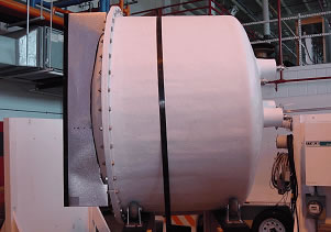
Figure
85 Side view
of calorimeter before it was mounted on the Sagebrush
Tracker. |
Vortek Solar Simulator
In
2003, the Vortek Simulator was fired up and operated reliably
on the calorimeter testing with FSEC’s
solar collector test apparatus. As expected, a few
computer and other problems delayed initial data
collection by a couple of days. However, these problems
were corrected and testing proceeded normally.
During
testing, the calorimeter was connected to the existing
facility’s hydronic loop, which was
developed over a period of years to a temperature
stability of 0.01 degrees centigrade. The irradiance
level measured about 820 watts per square meter over
an aperture of 0.557 square meters. The calorimeter
was tested as though it were a flat plate collector,
to obtain its efficiency curve. This was used to
infer the thermal losses and solar heat gain coefficient
of the eighth inch clear single pane of glass used
for the test. The nominal wind speed was set by the
laminar blower to five miles per hour. The coolant
flow was run at levels of 0.2, 0.5, and 1.0 gallons
per minute (GPM), and at varying inlet temperatures.
For all test runs, steady state conditions were established
by observing the outlet temperature in a real-time plot
as equilibrium was approached. During periods of non-equilibrium,
the recorded data was used to measure the first-order
system time constant, a function of the flow rate. The
calorimeter time constant varied from 1.5 minutes at
1.0 GPM to 6.9 minutes at 0.2 GPM. These time constants
were obtained by blocking the incident beam and watching
the decay in outlet temperature.
Skylight Dome Transmittance
Researchers completed work on the skylight dome transmittance,
adding a spherical shape to the cylindrical one previously
used. The ray tracing programming was changed to eliminate
reflection of rays approaching the dome from the inside,
for comparison with the analytical model, which does
not yet include internal reflections. The difference
between the two computational approaches, at a 30 E solar
zenith angle is 1.7%, considered acceptable for rating
skylight performance.
With both cylindrical and spherical dome models, transmittance
at large solar zenith angles above 60 is substantially
greater than for a horizontal flat plate. This is because
most of the rays incident on the dome and entering the
skylight are incident on the dome close to perpendicular,
where dome transmittance is highest.
Energy Gauge USA and Energy Gauge FlaRes
BAIHP mapped a table of window and shade characteristic
simulations that could be run with these two programs.
These runs will be used to determine the energy use of
various fenestration options for Florida residences and
to guide the preparation of instructional materials.
Florida Market Transformation
From the beginning of the BAIHP program, researchers
have provided technical background information and support
to the Alliance to Save Energy and the Efficient Windows
Collaborative to promote the sale and installation of
energy efficient fenestration in hot climates (such as
Florida) and other areas for both conventional and industrialized
homes. BAIHP also provides advice, technical information,
and educational information to energy companies regarding
window energy performance.
National Fenestration Rating Council (NFRC) Technical
Committee
In 2002, BAIHP presented a final report at a Task Group
meeting in Houston, on the NFRC- funded work to develop
a draft standard practice for the rating of tubular daylighting
devices. That project is now complete.
In
2001, BAIHP researchers performed a number of ray traces
on a highly reflective cylinder of varying lengths, using
the trace results to determine the cylinder’s
transmittances for different interior surface reflectivities
(from 90% to 100%). These results generated a “default
table” for determining the transmittance of this
tubular daylighting component. Using simplified assumptions,
and then multiplying the tube transmittance by the
top and bottom dome transmittance results, researchers
determined the total transmittance for a chosen sun
angle. Based on the findings, BAIHP provided NFRC and
the industry with a list of suggested research projects
to test and develop this methodology further. One of
these submitted projects was sent out for bid by ASHRAE
in Year 4 and is expected to begin in Year 5.
Tubular Daylighting Device SHGC and VT Value Calculations
Following a request from the TDD industry, a sequence
of operations and a new computer program were written
to access the Window 5 glazing database and obtain from
it the spectral transmittance and front and back reflectance
data for any sheet of glazing in that database which
might be used in making the top dome of a tubular daylighting
device. This permits determination of the input parameters
needed to run TDDTrans. The computer program was posted
for free download and is available by clicking on http://fsec.ucf.edu/download/br/fenestration/software/TddTrans-Beta/TDDTrans.exe .
Access sequence:
- Download and run the Optics 5 program.
- Select the glazing to be used in the tubular
daylighting device.
- Export its spectral data file as a standard
ASCII text file.
|


 You
are here: >
You
are here: > 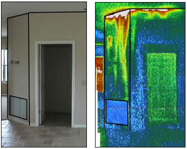